Characteristic Time with Details#
%load_ext autoreload
%autoreload 2
import numpy as np
import matplotlib.pyplot as plt
from matplotlib import colors
import seaborn as sns

from m3util.viz.style import set_style
from m3util.viz.printing import printer
from m3util.viz.layout import layout_fig
from sto_rheed.Dataset import RHEED_parameter_dataset
from sto_rheed.Viz import Viz
from sto_rheed.Analysis import analyze_curves, remove_outlier, smooth
from sto_rheed.Packed_functions import visualize_characteristic_time, violinplot_characteristic_time
from sto_rheed.Fit import NormalizeData

printing = printer(basepath = '../Figures/4.Characteristic_time/')
printing_plot = printer(basepath = '../Figures/4.Characteristic_time/', fileformats=['png', 'svg', 'tif'], dpi=600)

set_style("printing")

seq_colors = ['#00429d','#2e59a8','#4771b2','#5d8abd','#73a2c6','#8abccf','#a5d5d8','#c5eddf','#ffffe0']
bgc1, bgc2 = colors.hex2color(seq_colors[0]), colors.hex2color(seq_colors[5])
color_blue = (44/255,123/255,182/255)
color_orange = (217/255,95/255,2/255)
color_purple = (117/255,112/255,179/255)
printing set for seaborn
1. Examples of Fitted RHEED Intenstity Curve#
spot = 'spot_2'
metric = 'img_sum'
camera_freq = 500
fit_settings = {'savgol_window_order': (15, 3), 'pca_component': 10, 'I_diff': 15000,
                'unify':False, 'bounds':[0.001, 1], 'p_init':[0.1, 0.4, 0.1]}
2. Analyze the Decay Curve#
2.1 Sample 1 - treated_213nm#
2.1.1 Fitting Process#
path = 'D:/STO_STO-Data/RHEED/STO_STO_Berkeley/test6_gaussian_fit_parameters_all-04232023.h5'
D1_para = RHEED_parameter_dataset(path, camera_freq=500, sample_name='treated_213nm')
growth_list = ['growth_1', 'growth_2', 'growth_3', 'growth_4', 'growth_5']
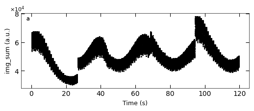
D1_para.viz_RHEED_parameter_trend(growth_list, spot='spot_2', metric_list=['img_sum'], head_tail=(100,300), interval=200)
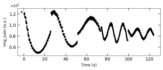
Gaussian fitted parameters in time: Fig. a: maximum intensity of original cropped RHEED spot, b: maximum intensity of resonstructed cropped RHEED spot, c: spot center in spot x coordinate, d: spot center in y coordinate, e: spot width in x coordinate, f: spot width in y coordinate.
growth_dict = {'growth_1':1, 'growth_2':1, 'growth_3':1, 'growth_4':3, 'growth_5':3}
x_all, y_all = D1_para.load_multiple_curves(growth_dict.keys(), spot, metric, x_start=0, interval=0)

parameters_all, x_coor_all, info = analyze_curves(D1_para, growth_dict, spot, metric, interval=0, fit_settings=fit_settings)
[xs_all, ys_all, ys_fit_all, ys_nor_all, ys_nor_fit_all, ys_nor_fit_failed_all, labels_all, losses_all] = info

# define two color regime
x_y1 = x_coor_all[losses_all[:,0]>losses_all[:,1]]
x_y2 = x_coor_all[losses_all[:,0]<losses_all[:,1]]
color_array = Viz.two_color_array(x_coor_all, x_y1, x_y2, bgc1, bgc2, transparency=0.5)
color_array = np.concatenate([np.expand_dims(x_coor_all, 1), color_array], axis=1)
Viz.plot_fit_details(xs_all, ys_nor_all, ys_nor_fit_all, ys_nor_fit_failed_all, labels=range(len(x_all)),
                     save_name='S10-fitting_details_treated_213nm', printing=printing_plot)
c:\users\yig319\lehigh university dropbox\yichen guo\predicting-pulsed-laser-deposition-srtio3-homoepitaxy-growth-dynamics-using-rheed\src\sto_rheed\Viz.py:565: UserWarning: The figure layout has changed to tight
  plt.tight_layout(pad=-0.5, w_pad=-1, h_pad=-0.5)
../Figures/4.Characteristic_time/S10-fitting_details_treated_213nm-1.png
../Figures/4.Characteristic_time/S10-fitting_details_treated_213nm-1.svg
../Figures/4.Characteristic_time/S10-fitting_details_treated_213nm-1.tif

../Figures/4.Characteristic_time/S10-fitting_details_treated_213nm-2.png
../Figures/4.Characteristic_time/S10-fitting_details_treated_213nm-2.svg
../Figures/4.Characteristic_time/S10-fitting_details_treated_213nm-2.tif

../Figures/4.Characteristic_time/S10-fitting_details_treated_213nm-3.png
../Figures/4.Characteristic_time/S10-fitting_details_treated_213nm-3.svg
../Figures/4.Characteristic_time/S10-fitting_details_treated_213nm-3.tif

../Figures/4.Characteristic_time/S10-fitting_details_treated_213nm-4.png
../Figures/4.Characteristic_time/S10-fitting_details_treated_213nm-4.svg
../Figures/4.Characteristic_time/S10-fitting_details_treated_213nm-4.tif

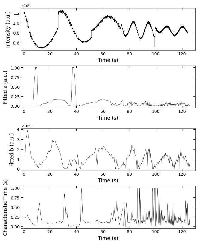
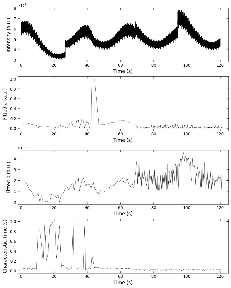
2.1.2 Fitted parameters#
fig, axes = layout_fig(4, 1, figsize=(6.5, 2*4))
Viz.plot_curve(axes[0], x_all, y_all, plot_type='lineplot', xlabel='Time (s)', ylabel='Intensity (a.u.)', xlim=(-2, 130), yaxis_style='sci')
Viz.plot_curve(axes[1], x_coor_all, parameters_all[:,0], plot_type='lineplot', xlabel='Time (s)', ylabel='Fitted a (a.u.)', xlim=(-2, 130))
Viz.plot_curve(axes[2], x_coor_all, parameters_all[:,1], plot_type='lineplot', xlabel='Time (s)', ylabel='Fitted b (a.u.)', xlim=(-2, 130))
Viz.plot_curve(axes[3], x_coor_all, parameters_all[:,2], plot_type='lineplot', xlabel='Time (s)', ylabel='Characteristic Time (s)', xlim=(-2, 130))
printing_plot.savefig(fig, 'S7-treated_213nm-a_b_tau')
plt.show()
C:\Users\yig319\Anaconda3\envs\test_rheed\Lib\site-packages\m3util\viz\layout.py:255: UserWarning: This figure was using a layout engine that is incompatible with subplots_adjust and/or tight_layout; not calling subplots_adjust.
  fig.subplots_adjust(wspace=wspace, hspace=hspace)
../Figures/4.Characteristic_time/S7-treated_213nm-a_b_tau.png
../Figures/4.Characteristic_time/S7-treated_213nm-a_b_tau.svg
../Figures/4.Characteristic_time/S7-treated_213nm-a_b_tau.tif
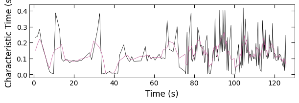
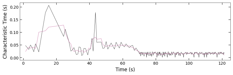
2.1.3 Remove Outliers#
Because there is hard boundary when characteristic >= 1, so we can assume the characteristic data that >= 0.95 are outliers and remove from plot. And we also process the data with less noise to observe the trend.
x_coor_all_clean, tau_clean = remove_outlier(x_coor_all, parameters_all[:,2], 0.95)
tau_smooth = smooth(tau_clean, 5)

x_coor_all_clean_sample1 = np.copy(x_coor_all_clean)
tau_clean_sample1 = np.copy(tau_clean)
tau_smooth_sample1 = np.copy(tau_smooth)

fig, ax = plt.subplots(1, 1, figsize=(6, 2), layout='compressed')
Viz.plot_curve(ax, x_coor_all_clean_sample1, tau_clean_sample1, curve_y_fit=tau_smooth_sample1, plot_type='lineplot',
            plot_colors=['k', '#bc5090'], xlabel='Time (s)', ylabel='Characteristic Time (s)',
            yaxis_style='linear', markersize=3, xlim=(-2, 130))
plt.show()
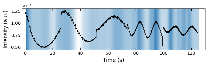
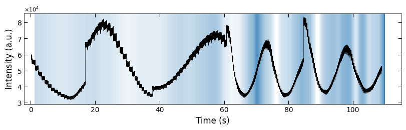
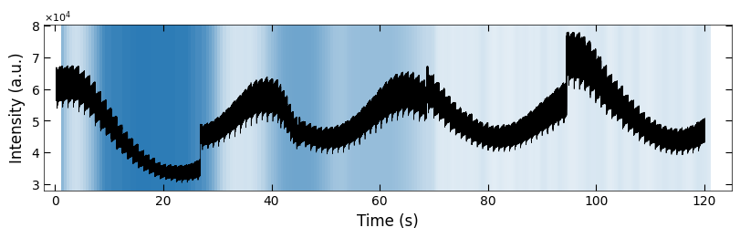
2.1.4 Plot with Background#
x_coor_all_clean, tau_clean = remove_outlier(x_coor_all, parameters_all[:,2], 0.95)
tau_smooth = smooth(tau_clean, 3)

x_FineStep, colors_all = Viz.make_fine_step(x_coor_all_clean, tau_smooth, step=2, color=color_blue, saturation=1, savgol_filter_level=(15, 3))
color_array = np.concatenate([np.expand_dims(x_FineStep, 1), colors_all], axis=1)

x_all_sample1 = np.copy(x_all)
y_all_sample1 = np.copy(y_all)
color_array_sample1 = np.copy(color_array)

fig, ax = plt.subplots(1, 1, figsize=(6.5, 2), layout='compressed')
Viz.draw_background_colors(ax, color_array_sample1)
ax.plot(x_all_sample1, y_all_sample1, color='k')
Viz.set_labels(ax, xlabel='Time (s)', ylabel='Intensity (a.u.)', title=None, xlim=(-2, 130))
plt.show()
np.save('../Data/Plume_results/treated_213nm-fitting_results(sklearn).npy', np.concatenate([np.expand_dims(x_coor_all, 1), parameters_all], axis=1))
np.save('../Data/Plume_results/treated_213nm-bg_tau.npy', color_array_sample1)
2.2 Sample 2 - treated_81nm#
2.2.1 Fitting process#
path = 'D:/STO_STO-Data/RHEED/STO_STO_Berkeley/test7_gaussian_fit_parameters_all-04232023.h5'
D2_para = RHEED_parameter_dataset(path, camera_freq=500, sample_name='treated_81nm')

growth_list = ['growth_1', 'growth_2', 'growth_3', 'growth_4', 'growth_5']
D2_para.viz_RHEED_parameter_trend(growth_list, spot='spot_2', metric_list=['img_sum'], head_tail=(100,300), interval=200)
Gaussian fitted parameters in time: Fig. a: maximum intensity of original cropped RHEED spot, b: maximum intensity of resonstructed cropped RHEED spot, c: spot center in spot x coordinate, d: spot center in y coordinate, e: spot width in x coordinate, f: spot width in y coordinate.
growth_dict = {'growth_1':1, 'growth_2':1, 'growth_3':1, 'growth_4':3, 'growth_5':3}
x_all, y_all = D2_para.load_multiple_curves(growth_dict.keys(), spot, metric, x_start=0, interval=0)

parameters_all, x_coor_all, info = analyze_curves(D2_para, growth_dict, spot, metric, interval=0, fit_settings=fit_settings)
[xs_all, ys_all, ys_fit_all, ys_nor_all, ys_nor_fit_all, ys_nor_fit_failed_all, labels_all, losses_all] = info

# define two color regime
x_y1 = x_coor_all[losses_all[:,0]>losses_all[:,1]]
x_y2 = x_coor_all[losses_all[:,0]<losses_all[:,1]]
color_array = Viz.two_color_array(x_coor_all, x_y1, x_y2, bgc1, bgc2, transparency=0.5)
color_array = np.concatenate([np.expand_dims(x_coor_all, 1), color_array], axis=1)
Viz.plot_fit_details(xs_all, ys_nor_all, ys_nor_fit_all, ys_nor_fit_failed_all, labels=range(len(x_all)),
                     save_name='S11-fitting_details_treated_81nm', printing=printing_plot)
c:\users\yig319\lehigh university dropbox\yichen guo\predicting-pulsed-laser-deposition-srtio3-homoepitaxy-growth-dynamics-using-rheed\src\sto_rheed\Viz.py:565: UserWarning: The figure layout has changed to tight
  plt.tight_layout(pad=-0.5, w_pad=-1, h_pad=-0.5)
../Figures/4.Characteristic_time/S11-fitting_details_treated_81nm-1.png
../Figures/4.Characteristic_time/S11-fitting_details_treated_81nm-1.svg
../Figures/4.Characteristic_time/S11-fitting_details_treated_81nm-1.tif

../Figures/4.Characteristic_time/S11-fitting_details_treated_81nm-2.png
../Figures/4.Characteristic_time/S11-fitting_details_treated_81nm-2.svg
../Figures/4.Characteristic_time/S11-fitting_details_treated_81nm-2.tif

../Figures/4.Characteristic_time/S11-fitting_details_treated_81nm-3.png
../Figures/4.Characteristic_time/S11-fitting_details_treated_81nm-3.svg
../Figures/4.Characteristic_time/S11-fitting_details_treated_81nm-3.tif

../Figures/4.Characteristic_time/S11-fitting_details_treated_81nm-4.png
../Figures/4.Characteristic_time/S11-fitting_details_treated_81nm-4.svg
../Figures/4.Characteristic_time/S11-fitting_details_treated_81nm-4.tif

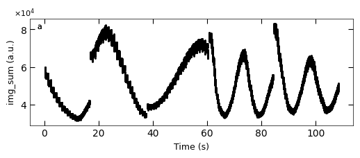
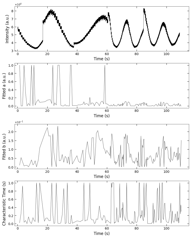
2.2.2 Fitted parameters#
fig, axes = layout_fig(4, 1, figsize=(8, 10))
Viz.plot_curve(axes[0], x_all, y_all, plot_type='lineplot', xlabel='Time (s)', ylabel='Intensity (a.u.)', xlim=(-2, 115), yaxis_style='sci')
Viz.plot_curve(axes[1], x_coor_all, parameters_all[:,0], plot_type='lineplot', xlabel='Time (s)', ylabel='Fitted a (a.u.)', xlim=(-2, 115))
Viz.plot_curve(axes[2], x_coor_all, parameters_all[:,1], plot_type='lineplot', xlabel='Time (s)', ylabel='Fitted b (a.u.)', xlim=(-2, 115))
Viz.plot_curve(axes[3], x_coor_all, parameters_all[:,2], plot_type='lineplot', xlabel='Time (s)', ylabel='Characteristic Time (s)', xlim=(-2, 115))
printing_plot.savefig(fig, 'S8-treated_81nm-a_b_tau')
plt.show()
C:\Users\yig319\Anaconda3\envs\test_rheed\Lib\site-packages\m3util\viz\layout.py:255: UserWarning: This figure was using a layout engine that is incompatible with subplots_adjust and/or tight_layout; not calling subplots_adjust.
  fig.subplots_adjust(wspace=wspace, hspace=hspace)
../Figures/4.Characteristic_time/S8-treated_81nm-a_b_tau.png
../Figures/4.Characteristic_time/S8-treated_81nm-a_b_tau.svg
../Figures/4.Characteristic_time/S8-treated_81nm-a_b_tau.tif
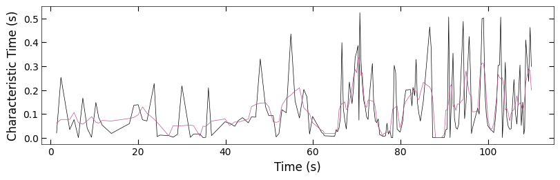
2.2.3 Remove Outliers#
Because there is hard boundary when characteristic >= 1, so we can assume the characteristic data that >= 0.95 are outliers and remove from plot. And we also process the data with less noise to observe the trend.
x_coor_all_clean, tau_clean = remove_outlier(x_coor_all, parameters_all[:,2], 0.95)
tau_smooth = smooth(tau_clean, 5)

x_coor_all_clean_sample2 = np.copy(x_coor_all_clean)
tau_clean_sample2 = np.copy(tau_clean)
tau_smooth_sample2 = np.copy(tau_smooth)

fig, ax = plt.subplots(1, 1, figsize=(8, 2.5), layout='compressed')
Viz.plot_curve(ax, x_coor_all_clean_sample2, tau_clean_sample2, curve_y_fit=tau_smooth_sample2, plot_type='lineplot',
           plot_colors=['k', '#bc5090'], xlabel='Time (s)', ylabel='Characteristic Time (s)',
           yaxis_style='linear', markersize=3, xlim=(-2, 115))
2.2.4 Plot with Background#
x_coor_all_clean, tau_clean = remove_outlier(x_coor_all, parameters_all[:,2], 0.95)
tau_smooth = smooth(tau_clean, 3)

x_FineStep, colors_all = Viz.make_fine_step(x_coor_all_clean, tau_smooth, step=2, color=color_blue, saturation=1, savgol_filter_level=(15, 3))
color_array = np.concatenate([np.expand_dims(x_FineStep, 1), colors_all], axis=1)

x_all_sample2 = np.copy(x_all)
y_all_sample2 = np.copy(y_all)
color_array_sample2 = np.copy(color_array)

fig, ax = plt.subplots(1, 1, figsize=(8, 2.5), layout='compressed')
Viz.draw_background_colors(ax, color_array_sample2)
ax.plot(x_all_sample2, y_all_sample2, color='k')
Viz.set_labels(ax, xlabel='Time (s)', ylabel='Intensity (a.u.)', title=None, xlim=(-2, 115))
plt.show()
np.save('../Data/Plume_results/treated_81nm-fitting_results(sklearn).npy', np.concatenate([np.expand_dims(x_coor_all, 1), parameters_all], axis=1))
np.save('../Data/Plume_results/treated_81nm-bg_tau.npy', color_array_sample2)
2.3 Sample 3 - untreated_162nm#
2.3.1 Fitting Process#
path = 'D:/STO_STO-Data/RHEED/STO_STO_Berkeley/test9_gaussian_fit_parameters_all-04232023.h5'
D3_para = RHEED_parameter_dataset(path, camera_freq=500, sample_name='untreated_162nm')

growth_list = ['growth_1', 'growth_2', 'growth_3', 'growth_4', 'growth_5']
D3_para.viz_RHEED_parameter_trend(growth_list, spot='spot_2', metric_list=['img_sum'], head_tail=(100,300), interval=200)
Gaussian fitted parameters in time: Fig. a: maximum intensity of original cropped RHEED spot, b: maximum intensity of resonstructed cropped RHEED spot, c: spot center in spot x coordinate, d: spot center in y coordinate, e: spot width in x coordinate, f: spot width in y coordinate.
growth_dict = {'growth_1':1, 'growth_2':1, 'growth_3':1, 'growth_4':3, 'growth_5':3}
x_all, y_all = D3_para.load_multiple_curves(growth_dict.keys(), spot, metric, x_start=0, interval=0)

parameters_all, x_coor_all, info = analyze_curves(D3_para, growth_dict, spot, metric, interval=0, fit_settings=fit_settings)
[xs_all, ys_all, ys_fit_all, ys_nor_all, ys_nor_fit_all, ys_nor_fit_failed_all, labels_all, losses_all] = info

# define two color regime
x_y1 = x_coor_all[losses_all[:,0]>losses_all[:,1]]
x_y2 = x_coor_all[losses_all[:,0]<losses_all[:,1]]
color_array = Viz.two_color_array(x_coor_all, x_y1, x_y2, bgc1, bgc2, transparency=0.5)
color_array = np.concatenate([np.expand_dims(x_coor_all, 1), color_array], axis=1)
Viz.plot_fit_details(xs_all, ys_nor_all, ys_nor_fit_all, ys_nor_fit_failed_all, labels=range(len(x_all)),
                     save_name='S12-fitting_details_untreated_162nm', printing=printing_plot)
c:\users\yig319\lehigh university dropbox\yichen guo\predicting-pulsed-laser-deposition-srtio3-homoepitaxy-growth-dynamics-using-rheed\src\sto_rheed\Viz.py:565: UserWarning: The figure layout has changed to tight
  plt.tight_layout(pad=-0.5, w_pad=-1, h_pad=-0.5)
../Figures/4.Characteristic_time/S12-fitting_details_untreated_162nm-1.png
../Figures/4.Characteristic_time/S12-fitting_details_untreated_162nm-1.svg
../Figures/4.Characteristic_time/S12-fitting_details_untreated_162nm-1.tif

../Figures/4.Characteristic_time/S12-fitting_details_untreated_162nm-2.png
../Figures/4.Characteristic_time/S12-fitting_details_untreated_162nm-2.svg
../Figures/4.Characteristic_time/S12-fitting_details_untreated_162nm-2.tif

../Figures/4.Characteristic_time/S12-fitting_details_untreated_162nm-3.png
../Figures/4.Characteristic_time/S12-fitting_details_untreated_162nm-3.svg
../Figures/4.Characteristic_time/S12-fitting_details_untreated_162nm-3.tif

../Figures/4.Characteristic_time/S12-fitting_details_untreated_162nm-4.png
../Figures/4.Characteristic_time/S12-fitting_details_untreated_162nm-4.svg
../Figures/4.Characteristic_time/S12-fitting_details_untreated_162nm-4.tif

../Figures/4.Characteristic_time/S12-fitting_details_untreated_162nm-5.png
../Figures/4.Characteristic_time/S12-fitting_details_untreated_162nm-5.svg
../Figures/4.Characteristic_time/S12-fitting_details_untreated_162nm-5.tif

2.3.2 Fitted parameters#
fig, axes = layout_fig(4, 1, figsize=(8, 10))
Viz.plot_curve(axes[0], x_all, y_all, plot_type='lineplot', xlabel='Time (s)', ylabel='Intensity (a.u.)', xlim=(-2, 125), yaxis_style='sci')
Viz.plot_curve(axes[1], x_coor_all, parameters_all[:,0], plot_type='lineplot', xlabel='Time (s)', ylabel='Fitted a (a.u.)', xlim=(-2, 125))
Viz.plot_curve(axes[2], x_coor_all, parameters_all[:,1], plot_type='lineplot', xlabel='Time (s)', ylabel='Fitted b (a.u.)', xlim=(-2, 125))
Viz.plot_curve(axes[3], x_coor_all, parameters_all[:,2], plot_type='lineplot', xlabel='Time (s)', ylabel='Characteristic Time (s)', xlim=(-2, 125))
printing_plot.savefig(fig, 'S9-untreated_162nm-a_b_tau')
plt.show()
C:\Users\yig319\Anaconda3\envs\test_rheed\Lib\site-packages\m3util\viz\layout.py:255: UserWarning: This figure was using a layout engine that is incompatible with subplots_adjust and/or tight_layout; not calling subplots_adjust.
  fig.subplots_adjust(wspace=wspace, hspace=hspace)
../Figures/4.Characteristic_time/S9-untreated_162nm-a_b_tau.png
../Figures/4.Characteristic_time/S9-untreated_162nm-a_b_tau.svg
../Figures/4.Characteristic_time/S9-untreated_162nm-a_b_tau.tif
2.3.3 Remove outliers#
Because there is hard boundary when characteristic >= 1, so we can assume the characteristic data that >= 0.95 are outliers and remove from plot. And we also process the data with less noise to observe the trend.
x_coor_all_clean, tau_clean = remove_outlier(x_coor_all, parameters_all[:,2], 0.95)
tau_smooth = smooth(tau_clean, 5)

x_coor_all_clean_sample3 = np.copy(x_coor_all_clean)
tau_clean_sample3 = np.copy(tau_clean)
tau_smooth_sample3 = np.copy(tau_smooth)
fig, ax = plt.subplots(1, 1, figsize=(8, 2.5), layout='compressed')
Viz.plot_curve(ax, x_coor_all_clean_sample3, tau_clean_sample3, curve_y_fit=tau_smooth_sample3, plot_type='lineplot',
           plot_colors=['k', '#bc5090'], xlabel='Time (s)', ylabel='Characteristic Time (s)',
           yaxis_style='linear', markersize=3, xlim=(-2, 125))
2.3.4 Plot with Background#
x_coor_all_clean, tau_clean = remove_outlier(x_coor_all, parameters_all[:,2], 0.95)
tau_smooth = smooth(tau_clean, 3)

x_FineStep, colors_all = Viz.make_fine_step(x_coor_all_clean, tau_smooth, step=2, color=color_blue, saturation=1, savgol_filter_level=(15, 3))
color_array = np.concatenate([np.expand_dims(x_FineStep, 1), colors_all], axis=1)

x_all_sample3 = np.copy(x_all)
y_all_sample3 = np.copy(y_all)
color_array_sample3 = np.copy(color_array)

fig, ax = plt.subplots(1, 1, figsize=(8, 2.5), layout='compressed')
Viz.draw_background_colors(ax, color_array_sample3)
ax.plot(x_all_sample3, y_all_sample3, color='k')
Viz.set_labels(ax, xlabel='Time (s)', ylabel='Intensity (a.u.)', title=None, xlim=(-2, 125))
plt.show()
np.save('../Data/Plume_results/untreated_162nm-fitting_results(sklearn).npy', np.concatenate([np.expand_dims(x_coor_all, 1), parameters_all], axis=1))
np.save('../Data/Plume_results/untreated_162nm-bg_tau.npy', color_array_sample3)
3. Summary of Figures#
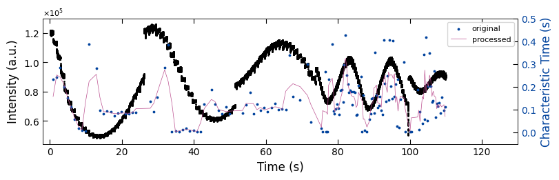
3.1 Plots of Characteristic Times with RHEED intensity#
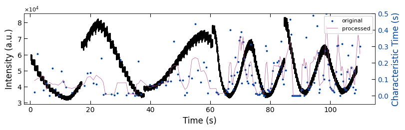
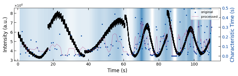
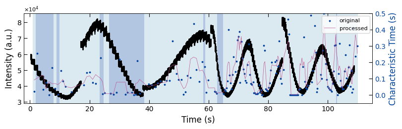
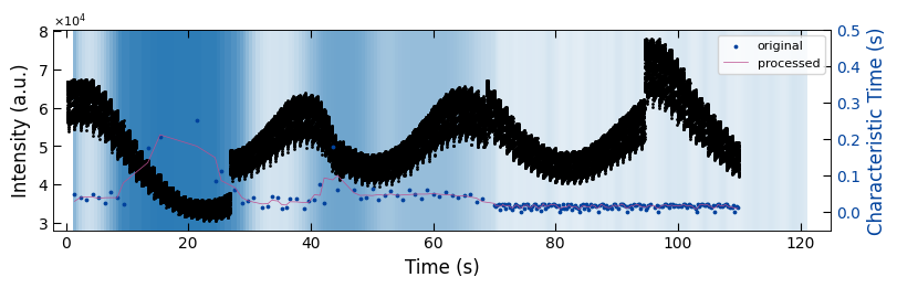
3.1.1 Sample 1 - treated_213nm#
x_all_sample1, y_all_sample1 = np.load('../Data/Plume_results/treated_213nm-x_all.npy'), np.load('../Data/Plume_results/treated_213nm-y_all.npy')
x_sklearn_sample1, tau_sklearn_sample1 = np.swapaxes(np.load('../Data/Plume_results/treated_213nm-fitting_results(sklearn).npy'), 0, 1)[[0, -1]]
bg_growth_sample1 = np.load('../Data/Plume_results/treated_213nm-bg_growth.npy')
bg_tau_sample1 = np.load('../Data/Plume_results/treated_213nm-bg_tau.npy')

y_all_sample1 = y_all_sample1[x_all_sample1<110]
x_all_sample1 = x_all_sample1[x_all_sample1<110]
tau_sklearn_sample1 = tau_sklearn_sample1[x_sklearn_sample1<110]
x_sklearn_sample1 = x_sklearn_sample1[x_sklearn_sample1<110]
bg_growth_sample1 = bg_growth_sample1[bg_growth_sample1[:, 0]<110]

x_sklearn_sample1, tau_clean_sample1 = remove_outlier(x_sklearn_sample1, tau_sklearn_sample1, 0.95)
tau_smooth_sample1 = smooth(tau_clean_sample1, 3)
fig, ax1 = plt.subplots(1, 1, figsize=(8, 2.5), layout='compressed')
ax1.scatter(x_all_sample1, y_all_sample1, color='k', s=1)
Viz.set_labels(ax1, xlabel='Time (s)', ylabel='Intensity (a.u.)', xlim=(-2, 130), ticks_both_sides=False)

ax2 = ax1.twinx()
ax2.scatter(x_sklearn_sample1, tau_clean_sample1, color=seq_colors[0], s=3)
ax2.plot(x_sklearn_sample1, tau_smooth_sample1, color='#bc5090', markersize=3)
Viz.set_labels(ax2, ylabel='Characteristic Time (s)', yaxis_style='lineplot', ylim=(-0.05, 0.5), ticks_both_sides=False)

# colors.hex2color(seq_colors[0])
ax2.tick_params(axis="y", color='k', labelcolor=seq_colors[0])
ax2.set_ylabel('Characteristic Time (s)', color=seq_colors[0])
# ax2.tick_params(axis="y", color='k', labelcolor=seq_colors[0])
# ax2.set_ylabel('Characteristic Time (s)', color=seq_colors[0])
plt.legend(['original', 'processed'], fontsize=8, loc="upper right", frameon=True)
printing_plot.savefig(fig, 'treated_213nm-no_bg')
plt.show()
../Figures/4.Characteristic_time/treated_213nm-no_bg.png
../Figures/4.Characteristic_time/treated_213nm-no_bg.svg
../Figures/4.Characteristic_time/treated_213nm-no_bg.tif
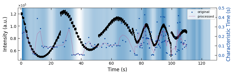
fig, ax1 = plt.subplots(1, 1, figsize=(8, 2.5), layout='compressed')
Viz.draw_background_colors(ax1, bg_tau_sample1)
ax1.scatter(x_all_sample1, y_all_sample1, color='k', s=1)
Viz.set_labels(ax1, xlabel='Time (s)', ylabel='Intensity (a.u.)', xlim=(-2, 130), ticks_both_sides=False)

ax2 = ax1.twinx()
ax2.scatter(x_sklearn_sample1, tau_clean_sample1, color=seq_colors[0], s=3)
ax2.plot(x_sklearn_sample1, tau_smooth_sample1, color='#bc5090', markersize=3)
Viz.set_labels(ax2, ylabel='Characteristic Time (s)', yaxis_style='lineplot', ylim=(-0.05, 0.5), ticks_both_sides=False)
ax2.tick_params(axis="y", color='k', labelcolor=seq_colors[0])
ax2.set_ylabel('Characteristic Time (s)', color=seq_colors[0])
plt.legend(['original', 'processed'], fontsize=8, loc="upper right", frameon=True)
printing_plot.savefig(fig, 'treated_213nm-tau_bg')
plt.show()
../Figures/4.Characteristic_time/treated_213nm-tau_bg.png
../Figures/4.Characteristic_time/treated_213nm-tau_bg.svg
../Figures/4.Characteristic_time/treated_213nm-tau_bg.tif
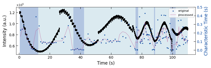
fig, ax1 = plt.subplots(1, 1, figsize=(8, 2.5), layout='compressed')
Viz.draw_background_colors(ax1, bg_growth_sample1)
ax1.scatter(x_all_sample1, y_all_sample1, color='k', s=1)
Viz.set_labels(ax1, xlabel='Time (s)', ylabel='Intensity (a.u.)', xlim=(-2, 130), ticks_both_sides=False)

ax2 = ax1.twinx()
ax2.scatter(x_sklearn_sample1, tau_clean_sample1, color=seq_colors[0], s=3)
ax2.plot(x_sklearn_sample1, tau_smooth_sample1, color='#bc5090', markersize=3)
Viz.set_labels(ax2, ylabel='Characteristic Time (s)', yaxis_style='lineplot', ylim=(-0.05, 0.5), ticks_both_sides=False)
ax2.tick_params(axis="y", color='k', labelcolor=seq_colors[0])
ax2.set_ylabel('Characteristic Time (s)', color=seq_colors[0])
plt.legend(['original', 'processed'], fontsize=8, loc="upper right", frameon=True)
plt.xlim(-2, 115)
printing_plot.savefig(fig, 'treated_213nm-growth_bg')
plt.show()
../Figures/4.Characteristic_time/treated_213nm-growth_bg.png
../Figures/4.Characteristic_time/treated_213nm-growth_bg.svg
../Figures/4.Characteristic_time/treated_213nm-growth_bg.tif
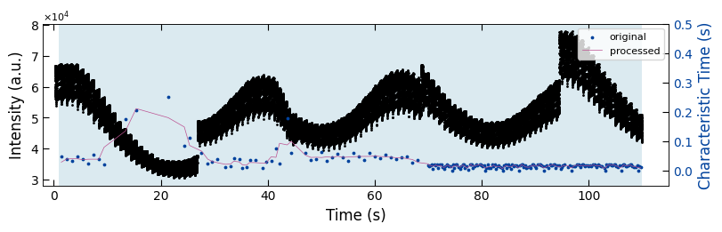
3.1.2 Sample 2 - treated_81nm#
x_all_sample2, y_all_sample2 = np.load('../Data/Plume_results/treated_81nm-x_all.npy'), np.load('../Data/Plume_results/treated_81nm-y_all.npy')
x_sklearn_sample2, tau_sklearn_sample2 = np.swapaxes(np.load('../Data/Plume_results/treated_81nm-fitting_results(sklearn).npy'), 0, 1)[[0, -1]]
bg_growth_sample2 = np.load('../Data/Plume_results/treated_81nm-bg_growth.npy')
bg_tau_sample2 = np.load('../Data/Plume_results/treated_81nm-bg_tau.npy')

y_all_sample2 = y_all_sample2[x_all_sample2<110]
x_all_sample2 = x_all_sample2[x_all_sample2<110]
tau_sklearn_sample2 = tau_sklearn_sample2[x_sklearn_sample2<110]
x_sklearn_sample2 = x_sklearn_sample2[x_sklearn_sample2<110]
bg_growth_sample2 = bg_growth_sample2[bg_growth_sample2[:, 0]<110]

x_sklearn_sample2, tau_clean_sample2 = remove_outlier(x_sklearn_sample2, tau_sklearn_sample2, 0.95)
tau_smooth_sample2 = smooth(tau_clean_sample2, 3)
fig, ax1 = plt.subplots(1, 1, figsize=(8, 2.5), layout='compressed')
ax1.scatter(x_all_sample2, y_all_sample2, color='k', s=1)
Viz.set_labels(ax1, xlabel='Time (s)', ylabel='Intensity (a.u.)', xlim=(-2, 115), ticks_both_sides=False)

ax2 = ax1.twinx()
ax2.scatter(x_sklearn_sample2, tau_clean_sample2, color=seq_colors[0], s=3)
ax2.plot(x_sklearn_sample2, tau_smooth_sample2, color='#bc5090', markersize=3)
Viz.set_labels(ax2, ylabel='Characteristic Time (s)', yaxis_style='lineplot', ylim=(-0.05, 0.5), ticks_both_sides=False)
ax2.tick_params(axis="y", color='k', labelcolor=seq_colors[0])
ax2.set_ylabel('Characteristic Time (s)', color=seq_colors[0])
plt.legend(['original', 'processed'], fontsize=8, loc="upper right", frameon=True)
printing_plot.savefig(fig, 'treated_81nm-no_bg')
plt.show()
../Figures/4.Characteristic_time/treated_81nm-no_bg.png
../Figures/4.Characteristic_time/treated_81nm-no_bg.svg
../Figures/4.Characteristic_time/treated_81nm-no_bg.tif
fig, ax1 = plt.subplots(1, 1, figsize=(8, 2.5), layout='compressed')
Viz.draw_background_colors(ax1, bg_tau_sample2)
ax1.scatter(x_all_sample2, y_all_sample2, color='k', s=1)
Viz.set_labels(ax1, xlabel='Time (s)', ylabel='Intensity (a.u.)', xlim=(-2, 115), ticks_both_sides=False)

ax2 = ax1.twinx()
ax2.scatter(x_sklearn_sample2, tau_clean_sample2, color=seq_colors[0], s=3)
ax2.plot(x_sklearn_sample2, tau_smooth_sample2, color='#bc5090', markersize=3)
Viz.set_labels(ax2, ylabel='Characteristic Time (s)', yaxis_style='lineplot', ylim=(-0.05, 0.5), ticks_both_sides=False)
ax2.tick_params(axis="y", color='k', labelcolor=seq_colors[0])
ax2.set_ylabel('Characteristic Time (s)', color=seq_colors[0])
plt.legend(['original', 'processed'], fontsize=8, loc="upper right", frameon=True)
printing_plot.savefig(fig, 'treated_81nm-tau_bg')
plt.show()
../Figures/4.Characteristic_time/treated_81nm-tau_bg.png
../Figures/4.Characteristic_time/treated_81nm-tau_bg.svg
../Figures/4.Characteristic_time/treated_81nm-tau_bg.tif
fig, ax1 = plt.subplots(1, 1, figsize=(8, 2.5), layout='compressed')
Viz.draw_background_colors(ax1, bg_growth_sample2)
ax1.scatter(x_all_sample2, y_all_sample2, color='k', s=1)
Viz.set_labels(ax1, xlabel='Time (s)', ylabel='Intensity (a.u.)', xlim=(-2, 115), ticks_both_sides=False)

ax2 = ax1.twinx()
ax2.scatter(x_sklearn_sample2, tau_clean_sample2, color=seq_colors[0], s=3)
ax2.plot(x_sklearn_sample2, tau_smooth_sample2, color='#bc5090', markersize=3)
Viz.set_labels(ax2, ylabel='Characteristic Time (s)', yaxis_style='lineplot', ylim=(-0.05, 0.5), ticks_both_sides=False)
ax2.tick_params(axis="y", color='k', labelcolor=seq_colors[0])
ax2.set_ylabel('Characteristic Time (s)', color=seq_colors[0])
plt.legend(['original', 'processed'], fontsize=8, loc="upper right", frameon=True)
plt.xlim(-2, 115)
printing_plot.savefig(fig, 'treated_81nm-growth_bg')
plt.show()
../Figures/4.Characteristic_time/treated_81nm-growth_bg.png
../Figures/4.Characteristic_time/treated_81nm-growth_bg.svg
../Figures/4.Characteristic_time/treated_81nm-growth_bg.tif
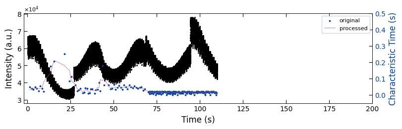
3.1.3 Sample 3 - untreated_162nm#
x_all_sample3, y_all_sample3 = np.load('../Data/Plume_results/untreated_162nm-x_all.npy'), np.load('../Data/Plume_results/untreated_162nm-y_all.npy')
x_sklearn_sample3, tau_sklearn_sample3 = np.swapaxes(np.load('../Data/Plume_results/untreated_162nm-fitting_results(sklearn).npy'), 0, 1)[[0, -1]]
bg_growth_sample3 = np.load('../Data/Plume_results/untreated_162nm-bg_growth.npy')
bg_tau_sample3 = np.load('../Data/Plume_results/untreated_162nm-bg_tau.npy')

y_all_sample3 = y_all_sample3[x_all_sample3<110]
x_all_sample3 = x_all_sample3[x_all_sample3<110]
tau_sklearn_sample3 = tau_sklearn_sample3[x_sklearn_sample3<110]
x_sklearn_sample3 = x_sklearn_sample3[x_sklearn_sample3<110]
bg_growth_sample3 = bg_growth_sample3[bg_growth_sample3[:, 0]<110]

x_sklearn_sample3, tau_clean_sample3 = remove_outlier(x_sklearn_sample3, tau_sklearn_sample3, 0.95)
tau_smooth_sample3 = smooth(tau_clean_sample3, 3)
fig, ax1 = plt.subplots(1, 1, figsize=(8, 2.5), layout='compressed')
ax1.scatter(x_all_sample3, y_all_sample3, color='k', s=1)
Viz.set_labels(ax1, xlabel='Time (s)', ylabel='Intensity (a.u.)', xlim=(-2, 200), ticks_both_sides=False)

ax2 = ax1.twinx()
ax2.scatter(x_sklearn_sample3, tau_clean_sample3, color=seq_colors[0], s=3)
ax2.plot(x_sklearn_sample3, tau_smooth_sample3, color='#bc5090', markersize=3)
Viz.set_labels(ax2, ylabel='Characteristic Time (s)', yaxis_style='lineplot', ylim=(-0.05, 0.5), ticks_both_sides=False)
ax2.tick_params(axis="y", color='k', labelcolor=seq_colors[0])
ax2.set_ylabel('Characteristic Time (s)', color=seq_colors[0])
plt.legend(['original', 'processed'], fontsize=8, loc="upper right", frameon=True)
printing_plot.savefig(fig, 'untreated_162nm-no_bg')
plt.show()
../Figures/4.Characteristic_time/untreated_162nm-no_bg.png
../Figures/4.Characteristic_time/untreated_162nm-no_bg.svg
../Figures/4.Characteristic_time/untreated_162nm-no_bg.tif
fig, ax1 = plt.subplots(1, 1, figsize=(8, 2.5), layout='compressed')
Viz.draw_background_colors(ax1, bg_tau_sample3)
ax1.scatter(x_all_sample3, y_all_sample3, color='k', s=1)
Viz.set_labels(ax1, xlabel='Time (s)', ylabel='Intensity (a.u.)', xlim=(-2, 125), ticks_both_sides=False)

ax2 = ax1.twinx()
ax2.scatter(x_sklearn_sample3, tau_clean_sample3, color=seq_colors[0], s=3)
ax2.plot(x_sklearn_sample3, tau_smooth_sample3, color='#bc5090', markersize=3)
Viz.set_labels(ax2, ylabel='Characteristic Time (s)', yaxis_style='lineplot', ylim=(-0.05, 0.5), ticks_both_sides=False)
ax2.tick_params(axis="y", color='k', labelcolor=seq_colors[0])
ax2.set_ylabel('Characteristic Time (s)', color=seq_colors[0])
plt.legend(['original', 'processed'], fontsize=8, loc="upper right", frameon=True)
printing_plot.savefig(fig, 'untreated_162nm-tau_bg')
plt.show()
../Figures/4.Characteristic_time/untreated_162nm-tau_bg.png
../Figures/4.Characteristic_time/untreated_162nm-tau_bg.svg
../Figures/4.Characteristic_time/untreated_162nm-tau_bg.tif
fig, ax1 = plt.subplots(1, 1, figsize=(8, 2.5), layout='compressed')
Viz.draw_background_colors(ax1, bg_growth_sample3)
ax1.scatter(x_all_sample3, y_all_sample3, color='k', s=1)
Viz.set_labels(ax1, xlabel='Time (s)', ylabel='Intensity (a.u.)', xlim=(-2, 125), ticks_both_sides=False)

ax2 = ax1.twinx()
ax2.scatter(x_sklearn_sample3, tau_clean_sample3, color=seq_colors[0], s=3)
# ax2.plot(x_sklearn_sample3, tau_smooth_sample3, color='#bc5090', markersize=3)
ax2.plot(x_sklearn_sample3, tau_smooth_sample3, color='#bc5090', markersize=3)
Viz.set_labels(ax2, ylabel='Characteristic Time (s)', yaxis_style='lineplot', ylim=(-0.05, 0.5), ticks_both_sides=False)
ax2.tick_params(axis="y", color='k', labelcolor=seq_colors[0])
ax2.set_ylabel('Characteristic Time (s)', color=seq_colors[0])
plt.legend(['original', 'processed'], fontsize=8, loc="upper right", frameon=True)
plt.xlim(-2, 115)
printing_plot.savefig(fig, 'untreated_162nm-growth_bg')
plt.show()
../Figures/4.Characteristic_time/untreated_162nm-growth_bg.png
../Figures/4.Characteristic_time/untreated_162nm-growth_bg.svg
../Figures/4.Characteristic_time/untreated_162nm-growth_bg.tif
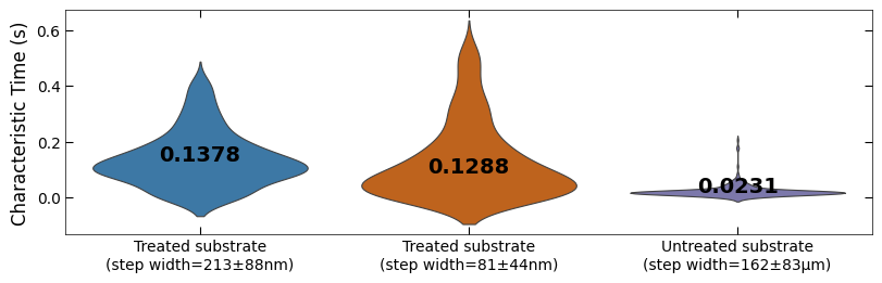
3.2 Violin Plot#
x_sklearn_sample1, tau_sklearn_sample1
(array([  0.958,   1.958,   2.958,   3.958,   4.958,   5.958,   6.958,
          7.958,   8.958,   9.958,  10.958,  12.958,  13.958,  14.958,
         15.958,  16.956,  17.958,  18.956,  19.958,  20.956,  21.956,
         22.958,  23.956,  27.922,  28.924,  29.922,  31.924,  32.924,
         33.924,  34.924,  35.924,  36.924,  37.924,  38.924,  39.924,
         40.922,  41.926,  42.924,  44.922,  45.922,  46.922,  47.922,
         48.918,  49.922,  53.558,  54.554,  55.688,  56.556,  57.55 ,
         58.556,  59.554,  60.556,  61.554,  62.554,  63.556,  64.556,
         65.556,  66.554,  67.556,  69.554,  71.554,  72.556,  75.478,
         75.81 ,  76.474,  76.806,  77.14 ,  77.47 ,  78.466,  78.796,
         79.13 ,  79.462,  79.792,  80.126,  80.458,  80.79 ,  81.116,
         81.454,  81.786,  82.112,  82.446,  82.782,  83.114,  83.446,
         83.778,  84.11 ,  84.442,  84.774,  85.108,  85.44 ,  85.77 ,
         86.434,  86.766,  87.098,  87.43 ,  88.094,  88.758,  89.092,
         89.422,  89.754,  90.088,  90.418,  90.746,  91.082,  91.414,
         91.746,  92.078,  92.41 ,  92.754,  93.086,  93.406,  93.75 ,
         94.086,  94.398,  94.734,  95.066,  95.398,  95.73 ,  96.062,
         96.396,  96.728,  97.06 ,  97.392,  98.388,  98.72 , 100.048,
        100.39 , 102.176, 102.508, 102.84 , 103.504, 103.836, 104.168,
        104.496, 104.832, 105.164, 105.492, 105.826, 106.16 , 106.492,
        106.824, 107.156, 107.488, 107.82 , 108.152, 108.484, 108.818,
        109.48 , 109.812]),
 array([0.23252341, 0.24057749, 0.2838626 , 0.19987291, 0.15164471,
        0.11260134, 0.05862685, 0.01770303, 0.00783538, 0.00532878,
        0.38733076, 0.60298316, 0.28053504, 0.09714899, 0.08247379,
        0.09496998, 0.09169998, 0.07287264, 0.08365561, 0.0895158 ,
        0.08282742, 0.08206836, 0.08731658, 0.08853761, 0.13710673,
        0.09214244, 0.15553819, 0.84366676, 0.28459062, 0.38299816,
        0.00186647, 0.0069553 , 0.00211146, 0.01187853, 0.01922647,
        0.00724996, 0.00838408, 0.00390978, 0.00238197, 0.12405537,
        0.98848516, 0.18636344, 0.12378757, 0.09576168, 0.0803125 ,
        0.11270139, 0.08275772, 0.08477307, 0.12226506, 0.17585872,
        0.08068095, 0.12328223, 0.09606673, 0.10976389, 0.08947116,
        0.10981278, 0.12673928, 0.1001355 , 0.10422678, 0.09962211,
        0.33872673, 0.1586782 , 0.49217207, 0.14333891, 0.64929001,
        0.30008074, 0.04662981, 0.48908013, 0.01808734, 0.00209139,
        0.57323786, 0.26636545, 0.00220417, 0.00233717, 0.23403352,
        0.62105611, 0.48246618, 0.38696555, 0.09247561, 0.08119167,
        0.10217687, 0.12296702, 0.10614699, 0.07942161, 0.18466538,
        0.18637748, 0.13204358, 0.29598448, 0.42636315, 0.25180346,
        0.21056782, 0.17622898, 0.18586466, 0.17789853, 0.11976332,
        0.1779569 , 0.17688728, 0.07465226, 0.07795532, 0.20523779,
        0.99999607, 0.24581312, 0.00216266, 0.16291452, 0.00884749,
        1.        , 0.00296229, 0.69811435, 0.05909249, 0.08301599,
        0.14799572, 0.15221784, 0.08389599, 0.35133031, 0.16318574,
        0.10969597, 0.11852723, 0.15885329, 0.09565996, 0.07786249,
        0.4040731 , 0.21359054, 0.13732333, 0.24741966, 0.14212866,
        0.40537347, 0.20266366, 0.14903737, 0.40271914, 0.15776179,
        0.21143361, 0.02605133, 0.23286041, 0.02266262, 0.14459961,
        1.        , 0.82787891, 0.30943413, 0.00200326, 0.99999991,
        1.        , 1.        , 0.00205021, 0.00193148, 1.        ,
        0.75898112, 0.18769659, 0.01288058, 0.09121558, 0.74685917,
        0.03980378, 0.34261041, 0.0576526 , 0.41877484, 0.05103715,
        0.20333042, 0.34890889, 0.2014184 , 0.13425987, 0.13835822,
        0.26960391, 0.06817423, 0.12808461, 0.11566498, 0.12967641,
        0.08469744, 0.15512118, 0.58887372, 0.09679319, 0.11305447]))
x_all_sample1, y_all_sample1 = np.load('../Data/Plume_results/treated_213nm-x_all.npy'), np.load('../Data/Plume_results/treated_213nm-y_all.npy')
x_sklearn_sample1, tau_sklearn_sample1 = np.swapaxes(np.load('../Data/Plume_results/treated_213nm-fitting_results(sklearn).npy'), 0, 1)[[0, -1]]
bg_growth_sample1 = np.load('../Data/Plume_results/treated_213nm-bg_growth.npy')
bg_tau_sample1 = np.load('../Data/Plume_results/treated_213nm-bg_tau.npy')

# y_all_sample1 = y_all_sample1[x_all_sample1<110]
# x_all_sample1 = x_all_sample1[x_all_sample1<110]
# tau_sklearn_sample1 = tau_sklearn_sample1[x_sklearn_sample1<110]
# x_sklearn_sample1 = x_sklearn_sample1[x_sklearn_sample1<110]
# bg_growth_sample1 = bg_growth_sample1[bg_growth_sample1[:, 0]<110]

x_sklearn_sample1, tau_clean_sample1 = remove_outlier(x_sklearn_sample1, tau_sklearn_sample1, 0.95)
tau_smooth_sample1 = smooth(tau_clean_sample1, 3)
x_all_sample2, y_all_sample2 = np.load('../Data/Plume_results/treated_81nm-x_all.npy'), np.load('../Data/Plume_results/treated_81nm-y_all.npy')
x_sklearn_sample2, tau_sklearn_sample2 = np.swapaxes(np.load('../Data/Plume_results/treated_81nm-fitting_results(sklearn).npy'), 0, 1)[[0, -1]]
bg_growth_sample2 = np.load('../Data/Plume_results/treated_81nm-bg_growth.npy')
bg_tau_sample2 = np.load('../Data/Plume_results/treated_81nm-bg_tau.npy')

# y_all_sample2 = y_all_sample2[x_all_sample2<110]
# x_all_sample2 = x_all_sample2[x_all_sample2<110]
# tau_sklearn_sample2 = tau_sklearn_sample2[x_sklearn_sample2<110]
# x_sklearn_sample2 = x_sklearn_sample2[x_sklearn_sample2<110]
# bg_growth_sample2 = bg_growth_sample2[bg_growth_sample2[:, 0]<110]

x_sklearn_sample2, tau_clean_sample2 = remove_outlier(x_sklearn_sample2, tau_sklearn_sample2, 0.9999)
tau_smooth_sample2 = smooth(tau_clean_sample2, 3)
x_all_sample3, y_all_sample3 = np.load('../Data/Plume_results/untreated_162nm-x_all.npy'), np.load('../Data/Plume_results/untreated_162nm-y_all.npy')
x_sklearn_sample3, tau_sklearn_sample3 = np.swapaxes(np.load('../Data/Plume_results/untreated_162nm-fitting_results(sklearn).npy'), 0, 1)[[0, -1]]
bg_growth_sample3 = np.load('../Data/Plume_results/untreated_162nm-bg_growth.npy')
bg_tau_sample3 = np.load('../Data/Plume_results/untreated_162nm-bg_tau.npy')

# y_all_sample3 = y_all_sample3[x_all_sample3<110]
# x_all_sample3 = x_all_sample3[x_all_sample3<110]
# tau_sklearn_sample3 = tau_sklearn_sample3[x_sklearn_sample3<110]
# x_sklearn_sample3 = x_sklearn_sample3[x_sklearn_sample3<110]
# bg_growth_sample3 = bg_growth_sample3[bg_growth_sample3[:, 0]<110]

x_sklearn_sample3, tau_clean_sample3 = remove_outlier(x_sklearn_sample3, tau_sklearn_sample3, 0.95)
tau_smooth_sample3 = smooth(tau_clean_sample3, 3)
fig, ax = plt.subplots(figsize=(8, 2.5), layout='compressed')
titles = ['Treated substrate\n(step width=213±88nm)',
          'Treated substrate\n(step width=81±44nm)',
          'Untreated substrate\n(step width=162±83μm)']

ax = sns.violinplot(data=[tau_clean_sample1, tau_clean_sample2, tau_clean_sample3],
                    palette=[color_blue, color_orange, color_purple], linewidth=0.8, inner=None)
Viz.set_labels(ax, ylabel='Characteristic Time (s)', ticks_both_sides=False, yaxis_style='linear')
Viz.label_violinplot(ax, [tau_clean_sample1, tau_clean_sample2, tau_clean_sample3], label_type='median', text_pos='center')
ax.set_xticklabels(titles)
printing.savefig(fig, 'violinplot_plot')
plt.show()
C:\Users\yig319\AppData\Local\Temp\ipykernel_33280\1078332159.py:10: UserWarning: set_ticklabels() should only be used with a fixed number of ticks, i.e. after set_ticks() or using a FixedLocator.
  ax.set_xticklabels(titles)
../Figures/4.Characteristic_time/violinplot_plot.png
../Figures/4.Characteristic_time/violinplot_plot.svg

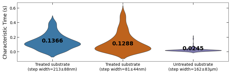
fig, ax = plt.subplots(figsize=(8, 2.5), layout='compressed')
titles = ['Treated substrate\n(step width=213±88nm)',
          'Treated substrate\n(step width=81±44nm)',
          'Untreated substrate\n(step width=162±83μm)']

ax = sns.violinplot(data=[tau_clean_sample1, tau_clean_sample2, tau_clean_sample3],
                    palette=[color_blue, color_orange, color_purple], linewidth=0.8, inner=None)
Viz.set_labels(ax, ylabel='Characteristic Time (s)', ticks_both_sides=False, yaxis_style='linear')
Viz.label_violinplot(ax, [tau_clean_sample1, tau_clean_sample2, tau_clean_sample3], label_type='average', text_pos='center')
ax.set_xticklabels(titles)
printing.savefig(fig, 'violinplot_plot')
plt.show()
C:\Users\yig319\AppData\Local\Temp\ipykernel_33280\3436764359.py:10: UserWarning: set_ticklabels() should only be used with a fixed number of ticks, i.e. after set_ticks() or using a FixedLocator.
  ax.set_xticklabels(titles)
../Figures/4.Characteristic_time/violinplot_plot.png
../Figures/4.Characteristic_time/violinplot_plot.svg
# align the data with time
tau_clean_sample1 = tau_clean_sample1[x_sklearn_sample1<110]
x_sklearn_sample1 = x_sklearn_sample1[x_sklearn_sample1<110]

tau_clean_sample2 = tau_clean_sample2[x_sklearn_sample2<110]
x_sklearn_sample2 = x_sklearn_sample2[x_sklearn_sample2<110]

tau_clean_sample3 = tau_clean_sample3[x_sklearn_sample3<110]
x_sklearn_sample3 = x_sklearn_sample3[x_sklearn_sample3<110]
fig, ax = plt.subplots(figsize=(8, 2.5), layout='compressed')
titles = ['Treated substrate\n(step width=213±88nm)',
          'Treated substrate\n(step width=81±44nm)',
          'Untreated substrate\n(step width=162±83μm)']

ax = sns.violinplot(data=[tau_clean_sample1, tau_clean_sample2, tau_clean_sample3],
                    palette=[color_blue, color_orange, color_purple], linewidth=0.8, inner=None)
Viz.set_labels(ax, ylabel='Characteristic Time (s)', ticks_both_sides=False, yaxis_style='linear')
Viz.label_violinplot(ax, [tau_clean_sample1, tau_clean_sample2, tau_clean_sample3], label_type='average', text_pos='center')
ax.set_xticklabels(titles)
printing.savefig(fig, 'violinplot_plot')
plt.show()
C:\Users\yig319\AppData\Local\Temp\ipykernel_33280\3436764359.py:10: UserWarning: set_ticklabels() should only be used with a fixed number of ticks, i.e. after set_ticks() or using a FixedLocator.
  ax.set_xticklabels(titles)
../Figures/4.Characteristic_time/violinplot_plot.png
../Figures/4.Characteristic_time/violinplot_plot.svg
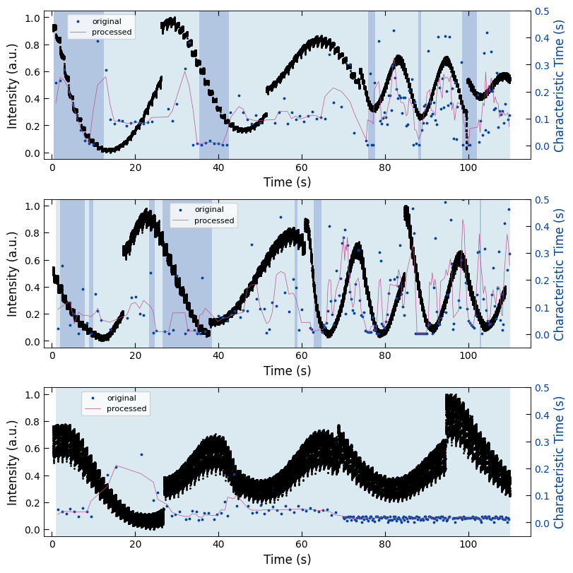
3.3 Summary Figure#
align_time = True
normalize = True

seq_colors = ['#00429d','#2e59a8','#4771b2','#5d8abd','#73a2c6','#8abccf','#a5d5d8','#c5eddf','#ffffe0']
fig, axes = layout_fig(3, 1, figsize=(8, 8))
ax1, ax3, ax5 = axes[0], axes[1], axes[2]

x_all_sample1, y_all_sample1 = np.load('../Data/Plume_results/treated_213nm-x_all.npy'), np.load('../Data/Plume_results/treated_213nm-y_all.npy')
x_sklearn_sample1, tau_sklearn_sample1 = np.swapaxes(np.load('../Data/Plume_results/treated_213nm-fitting_results(sklearn).npy'), 0, 1)[[0, -1]]
bg_growth_sample1 = np.load('../Data/Plume_results/treated_213nm-bg_growth.npy')

x_all_sample2, y_all_sample2 = np.load('../Data/Plume_results/treated_81nm-x_all.npy'), np.load('../Data/Plume_results/treated_81nm-y_all.npy')
x_sklearn_sample2, tau_sklearn_sample2 = np.swapaxes(np.load('../Data/Plume_results/treated_81nm-fitting_results(sklearn).npy'), 0, 1)[[0, -1]]
bg_growth_sample2 = np.load('../Data/Plume_results/treated_81nm-bg_growth.npy')

x_all_sample3, y_all_sample3 = np.load('../Data/Plume_results/untreated_162nm-x_all.npy'), np.load('../Data/Plume_results/untreated_162nm-y_all.npy')
x_sklearn_sample3, tau_sklearn_sample3 = np.swapaxes(np.load('../Data/Plume_results/untreated_162nm-fitting_results(sklearn).npy'), 0, 1)[[0, -1]]
bg_growth_sample3 = np.load('../Data/Plume_results/untreated_162nm-bg_growth.npy')


if align_time:
    y_all_sample1 = y_all_sample1[x_all_sample1<110]
    x_all_sample1 = x_all_sample1[x_all_sample1<110]
    tau_sklearn_sample1 = tau_sklearn_sample1[x_sklearn_sample1<110]
    x_sklearn_sample1 = x_sklearn_sample1[x_sklearn_sample1<110]
    bg_growth_sample1 = bg_growth_sample1[bg_growth_sample1[:, 0]<110]

    y_all_sample2 = y_all_sample2[x_all_sample2<110]
    x_all_sample2 = x_all_sample2[x_all_sample2<110]
    tau_sklearn_sample2 = tau_sklearn_sample2[x_sklearn_sample2<110]
    x_sklearn_sample2 = x_sklearn_sample2[x_sklearn_sample2<110]
    bg_growth_sample2 = bg_growth_sample2[bg_growth_sample2[:, 0]<110]

    y_all_sample3 = y_all_sample3[x_all_sample3<110]
    x_all_sample3 = x_all_sample3[x_all_sample3<110]
    tau_sklearn_sample3 = tau_sklearn_sample3[x_sklearn_sample3<110]
    x_sklearn_sample3 = x_sklearn_sample3[x_sklearn_sample3<110]
    bg_growth_sample3 = bg_growth_sample3[bg_growth_sample3[:, 0]<110]


if normalize:
    y_all_sample1 = NormalizeData(y_all_sample1, lb=np.min(y_all_sample1), ub=np.max(y_all_sample1))
    y_all_sample2 = NormalizeData(y_all_sample2, lb=np.min(y_all_sample2), ub=np.max(y_all_sample2))
    y_all_sample3 = NormalizeData(y_all_sample3, lb=np.min(y_all_sample3), ub=np.max(y_all_sample3))

x_sklearn_sample1, tau_clean_sample1 = remove_outlier(x_sklearn_sample1, tau_sklearn_sample1, 0.95)
tau_smooth_sample1 = smooth(tau_clean_sample1, 3)

x_sklearn_sample2, tau_clean_sample2 = remove_outlier(x_sklearn_sample2, tau_sklearn_sample2, 0.95)
tau_smooth_sample2 = smooth(tau_clean_sample2, 3)

x_sklearn_sample3, tau_clean_sample3 = remove_outlier(x_sklearn_sample3, tau_sklearn_sample3, 0.95)
tau_smooth_sample3 = smooth(tau_clean_sample3, 3)


Viz.draw_background_colors(ax1, bg_growth_sample1)
ax1.scatter(x_all_sample1, y_all_sample1, color='k', s=1)
Viz.set_labels(ax1, xlabel='Time (s)', ylabel='Intensity (a.u.)', xlim=(-2, 130), ticks_both_sides=False)

ax2 = ax1.twinx()
ax2.scatter(x_sklearn_sample1, tau_clean_sample1, color=seq_colors[0], s=3)
ax2.plot(x_sklearn_sample1, tau_smooth_sample1, color='#bc5090', markersize=3)
Viz.set_labels(ax2, ylabel='Characteristic Time (s)', yaxis_style='lineplot', ylim=(-0.05, 0.5), ticks_both_sides=False)
ax2.tick_params(axis="y", color='k', labelcolor=seq_colors[0])
ax2.set_ylabel('Characteristic Time (s)', color=seq_colors[0])
ax2.legend(['original', 'processed'], fontsize=8, loc="upper left", frameon=True, bbox_to_anchor=(0.04, 1))


Viz.draw_background_colors(ax3, bg_growth_sample2)
ax3.scatter(x_all_sample2, y_all_sample2, color='k', s=1)
Viz.set_labels(ax3, xlabel='Time (s)', ylabel='Intensity (a.u.)', xlim=(-2, 115), ticks_both_sides=False)

ax4 = ax3.twinx()
ax4.scatter(x_sklearn_sample2, tau_clean_sample2, color=seq_colors[0], s=3)
ax4.plot(x_sklearn_sample2, tau_smooth_sample2, color='#bc5090', markersize=3)
Viz.set_labels(ax4, ylabel='Characteristic Time (s)', yaxis_style='lineplot', ylim=(-0.05, 0.5), ticks_both_sides=False)
ax4.tick_params(axis="y", color='k', labelcolor=seq_colors[0])
ax4.set_ylabel('Characteristic Time (s)', color=seq_colors[0])
ax4.legend(['original', 'processed'], fontsize=8, loc="upper left", frameon=True, bbox_to_anchor=(0.25, 1))


Viz.draw_background_colors(ax5, bg_growth_sample3)
ax5.scatter(x_all_sample3, y_all_sample3, color='k', s=1)
Viz.set_labels(ax5, xlabel='Time (s)', ylabel='Intensity (a.u.)', xlim=(-2, 125), ticks_both_sides=False)

ax6 = ax5.twinx()
ax6.scatter(x_sklearn_sample3, tau_clean_sample3, color=seq_colors[0], s=3)
ax6.plot(x_sklearn_sample3, tau_smooth_sample3, color='#bc5090', markersize=3)
Viz.set_labels(ax6, ylabel='Characteristic Time (s)', yaxis_style='lineplot', ylim=(-0.05, 0.5), ticks_both_sides=False)
ax6.tick_params(axis="y", color='k', labelcolor=seq_colors[0])
ax6.set_ylabel('Characteristic Time (s)', color=seq_colors[0])
ax6.legend(['original', 'processed'], fontsize=8, loc="upper left", frameon=True, bbox_to_anchor=(0.07, 1))

if align_time:
    for ax in [ax1, ax2, ax3, ax4, ax5, ax6]:
        ax.set_xlim(-2, 115)

printing_plot.savefig(fig, 'growth_bg-characterization_time')
plt.show()
C:\Users\yig319\Anaconda3\envs\test_rheed\Lib\site-packages\m3util\viz\layout.py:255: UserWarning: This figure was using a layout engine that is incompatible with subplots_adjust and/or tight_layout; not calling subplots_adjust.
  fig.subplots_adjust(wspace=wspace, hspace=hspace)
../Figures/4.Characteristic_time/growth_bg-characterization_time.png
../Figures/4.Characteristic_time/growth_bg-characterization_time.svg
../Figures/4.Characteristic_time/growth_bg-characterization_time.tif