AFM and XRD with Details#
%load_ext autoreload
%autoreload 2
import os
import re
import numpy as np
import matplotlib.pyplot as plt
from m3util.viz.style import set_style
from m3util.viz.printing import printer
from m3util.viz.layout import layout_fig
from m3util.viz.text import labelfigs
from sto_rheed.AFM import visualize_afm_image, afm_substrate
from sto_rheed.XRD import plot_xrd, plot_rsm

# from be.Dataset import BE_Dataset
printing = printer(basepath = '../Figures/2.AFM_XRD/', fileformats=['png', 'svg', 'tif'], dpi=600)
set_style("printing")
printing set for seaborn
1. Download Datasets from Zenodo#
# # Download the Data file from Zenodo
# download=False
# if download:
#     # full size version
#     urls = ['https://zenodo.org/record/8000271/files/AFM.zip?download=1',
#             'https://zenodo.org/record/8000271/files/XRD.zip?download=1']

#     for url in urls:
#         # Specify the filename and the path to save the file
#         filename = re.split(r'\?', os.path.basename(url))[0]
#         save_path = './../2023_RHEED_PLD_SrTiO3/'

#         # download the file
#         download_and_unzip(filename, url, save_path)
# if os.path.isfile('../Data/AFM.zip'): os.remove('../Data/AFM.zip')
# if os.path.isfile('../Data/XRD.zip'): os.remove('../Data/XRD.zip')
2. AFM Results Analysis#
2.1 Sample 1 - treated_213nm#
2.1.1 Visualize and save the afm figures with colorbar and scalebar#
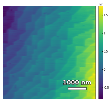
img1 = np.loadtxt('../Data/AFM/treated_213nm-substrate.txt')[:256]
scalebar_dict = {'image_size': 5000, 'scale_size': 1000, 'units': 'nm'}
visualize_afm_image(img1, colorbar_range=[-4e-10, 4e-10], figsize=(6,4), scalebar_dict=scalebar_dict,
                    filename='treated_213nm-substrate', printing=printing)
../Figures/2.AFM_XRD/treated_213nm-substrate.png
../Figures/2.AFM_XRD/treated_213nm-substrate.svg
../Figures/2.AFM_XRD/treated_213nm-substrate.tif

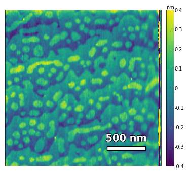
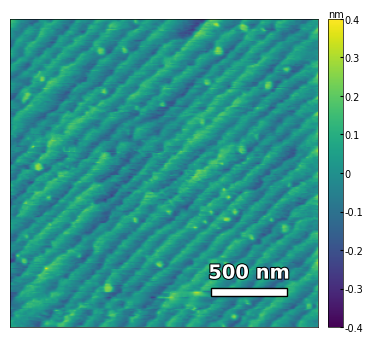
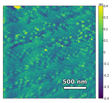
img2 = np.loadtxt('../Data/AFM/treated_213nm-film.txt')[:256]
scalebar_dict = {'image_size': 2008, 'scale_size': 500, 'units': 'nm'}
visualize_afm_image(img2, colorbar_range=[-4e-10, 4e-10], figsize=(6,4), scalebar_dict=scalebar_dict,
                    filename='treated_213nm-film', printing=printing)
../Figures/2.AFM_XRD/treated_213nm-film.png
../Figures/2.AFM_XRD/treated_213nm-film.svg
../Figures/2.AFM_XRD/treated_213nm-film.tif
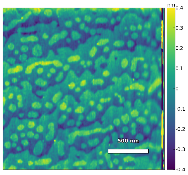
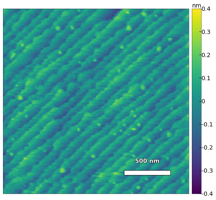
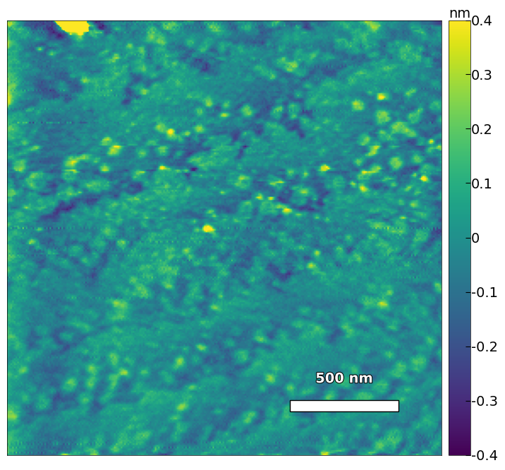
# high resolution image
img2 = np.loadtxt('../Data/AFM/treated_213nm-film.txt')[:256]
scalebar_dict = {'image_size': 2008, 'scale_size': 500, 'units': 'nm'}
visualize_afm_image(img2, colorbar_range=[-4e-10, 4e-10], figsize=(12,8), scalebar_dict=scalebar_dict,
                    filename='treated_213nm-film-high_res', printing=printing)
../Figures/2.AFM_XRD/treated_213nm-film-high_res.png
../Figures/2.AFM_XRD/treated_213nm-film-high_res.svg
../Figures/2.AFM_XRD/treated_213nm-film-high_res.tif
2.1.2 Calculate the substrate step height, step width, and miscut#
img3 = np.loadtxt('../Data/AFM/treated_213nm-substrate-tilted.txt')[:256]

scalebar_dict = {'image_size': 5000, 'scale_size': 1000, 'units': 'nm'}
visualize_afm_image(img3, colorbar_range=None, figsize=(6,4), scalebar_dict=scalebar_dict)
# rotate the angle to make step edges horizontal
analyzer = afm_substrate(img3, pixels=256, size=5e-6)
img_rot, size_rot = analyzer.rotate_image(angle=-50)

x, z, peak_indices, valley_indices = analyzer.slice_rotate(img_rot, size_rot, j=60, prominence=1e-5, width=2, xz_angle=3, demo=True)
# with the provided height from literature
step_heights, step_widths, miscut = analyzer.calculate_simple(x, z, peak_indices, fixed_height=3.91e-10, demo=True)
step_heights, step_widths, miscut = analyzer.calculate_substrate_properties(img_rot, size_rot, xz_angle=3, prominence=1e-3, width=2, style='simple', fixed_height=3.91e-10, std_range=1, demo=False)
Step 1: Height = 3.91e-10, Width = 1.62e-07, Miscut = 0.138°
Step 2: Height = 3.91e-10, Width = 1.40e-07, Miscut = 0.160°
Step 3: Height = 3.91e-10, Width = 1.08e-07, Miscut = 0.208°
Step 4: Height = 3.91e-10, Width = 9.57e-08, Miscut = 0.234°
Step 5: Height = 3.91e-10, Width = 1.94e-07, Miscut = 0.115°
Step 6: Height = 3.91e-10, Width = 1.71e-07, Miscut = 0.131°
Step 7: Height = 3.91e-10, Width = 3.99e-08, Miscut = 0.561°
Step 8: Height = 3.91e-10, Width = 1.23e-07, Miscut = 0.183°
Step 9: Height = 3.91e-10, Width = 2.11e-07, Miscut = 0.106°
Results:
  Average step height = 3.91e-10, Standard deviation = 0.00e+00
  Average step width = 1.38e-07, Standard deviation = 5.03e-08
  Average miscut = 0.204°, Standard deviation = 0.132°
Step height = 3.91e-10 +- 0.00e+00
Step width = 2.13e-07 +- 8.87e-08
Miscut = 0.131° +- 0.074°
# calculate the height from afm figure
step_heights, step_widths, miscut = analyzer.calculate_simple(x, z, peak_indices, demo=True)
step_heights, step_widths, miscut = analyzer.calculate_substrate_properties(img_rot, size_rot, xz_angle=3, prominence=1e-10, width=2, style='simple', std_range=1, demo=False)
Step 1: Height = 1.73e-10, Width = 1.62e-07, Miscut = 0.061°
Step 2: Height = 1.21e-10, Width = 1.40e-07, Miscut = 0.050°
Step 3: Height = -1.00e-10, Width = 1.08e-07, Miscut = -0.053°
Step 4: Height = 1.45e-10, Width = 9.57e-08, Miscut = 0.087°
Step 5: Height = 1.32e-10, Width = 1.94e-07, Miscut = 0.039°
Step 6: Height = 8.74e-11, Width = 1.71e-07, Miscut = 0.029°
Step 7: Height = 1.63e-11, Width = 3.99e-08, Miscut = 0.023°
Step 8: Height = 2.25e-11, Width = 1.23e-07, Miscut = 0.011°
Step 9: Height = 1.05e-10, Width = 2.11e-07, Miscut = 0.029°
Results:
  Average step height = 7.79e-11, Standard deviation = 8.01e-11
  Average step width = 1.38e-07, Standard deviation = 5.03e-08
  Average miscut = 0.031°, Standard deviation = 0.037°
Step height = 1.50e-10 +- 1.28e-10
Step width = 2.13e-07 +- 8.87e-08
Miscut = 0.042° +- 0.038°
x, z, peak_indices, valley_indices = analyzer.slice_rotate(img_rot, size_rot, j=100, prominence=1e-11, width=2, xz_angle=0, demo=True)
step_heights, step_widths, miscut = analyzer.calculate_fit(x, z, peak_indices, valley_indices, fixed_height=3.91e-10, demo=True)
step 1: step_width: 1.10e-10, left_peak: (4.99e-07, -4.60e-10), valley: (5.41e-07, -5.11e-10), right_peak: (6.93e-07, -2.94e-10)
step 2: step_width: 4.97e-10, left_peak: (6.93e-07, -2.94e-10), valley: (8.18e-07, -3.74e-10), right_peak: (8.87e-07, -1.42e-10)
step 3: step_width: 2.44e-10, left_peak: (9.57e-07, -1.84e-10), valley: (1.03e-06, -2.97e-10), right_peak: (1.15e-06, -6.09e-11)
step 4: step_width: 2.04e-10, left_peak: (1.33e-06, 1.19e-10), valley: (1.40e-06, 2.98e-11), right_peak: (1.52e-06, 2.37e-10)
step 5: step_width: 2.84e-10, left_peak: (1.52e-06, 2.37e-10), valley: (1.58e-06, 1.46e-10), right_peak: (1.65e-06, 3.88e-10)
step 6: step_width: 3.97e-10, left_peak: (1.73e-06, 2.83e-10), valley: (1.87e-06, 1.73e-10), right_peak: (1.97e-06, 3.74e-10)
step 7: step_width: 5.13e-10, left_peak: (1.97e-06, 3.74e-10), valley: (2.11e-06, 1.85e-10), right_peak: (2.19e-06, 3.79e-10)
step 8: step_width: 2.68e-10, left_peak: (2.19e-06, 3.79e-10), valley: (2.26e-06, 3.16e-10), right_peak: (2.33e-06, 5.22e-10)
step 9: step_width: 4.10e-10, left_peak: (2.33e-06, 5.22e-10), valley: (2.41e-06, 4.52e-10), right_peak: (2.47e-06, 6.79e-10)
step 10: step_width: 4.29e-10, left_peak: (2.47e-06, 6.79e-10), valley: (2.63e-06, 5.62e-10), right_peak: (2.76e-06, 7.97e-10)
step 11: step_width: 2.41e-10, left_peak: (2.76e-06, 7.97e-10), valley: (2.81e-06, 7.03e-10), right_peak: (2.91e-06, 9.61e-10)
step 12: step_width: 5.79e-11, left_peak: (2.91e-06, 9.61e-10), valley: (2.94e-06, 9.25e-10), right_peak: (2.97e-06, 9.47e-10)
Results:
  Average step height = 3.91e-10, Standard deviation = 0.00e+00
  Average step width = 3.05e-10, Standard deviation = 1.40e-10
  Average miscut = 54.187°, Standard deviation = 13.357°
The “simple” method with provided step height gives a more accurate results for the step width and miscut:
Step height = 3.91e-10 +- 0.00e+00
Step width = 2.13e-07 +- 8.87e-08
Miscut = 0.131° +- 0.074°
2.2 Sample 2 - treated_81nm:#
2.2.1 Visualize and save the afm figures with colorbar and scalebar#
img1 = np.loadtxt('../Data/AFM/treated_81nm-substrate.txt')[:256]
scalebar_dict = {'image_size': 5000, 'scale_size': 1000, 'units': 'nm'}
visualize_afm_image(img1, colorbar_range=[-4e-10, 4e-10], figsize=(6,4), scalebar_dict=scalebar_dict,
                    filename='treated_81nm-substrate', printing=printing)
../Figures/2.AFM_XRD/treated_81nm-substrate.png
../Figures/2.AFM_XRD/treated_81nm-substrate.svg
../Figures/2.AFM_XRD/treated_81nm-substrate.tif
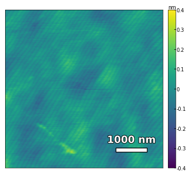
img2 = np.loadtxt('../Data/AFM/treated_81nm-film.txt')[:256]
scalebar_dict = {'image_size': 2008, 'scale_size': 500, 'units': 'nm'}
visualize_afm_image(img2, colorbar_range=[-4e-10, 4e-10], figsize=(6,4), scalebar_dict=scalebar_dict,
                    filename='treated_81nm-film', printing=printing)
../Figures/2.AFM_XRD/treated_81nm-film.png
../Figures/2.AFM_XRD/treated_81nm-film.svg
../Figures/2.AFM_XRD/treated_81nm-film.tif
img3 = np.loadtxt('../Data/AFM/treated_81nm-film.txt')[:256]
scalebar_dict = {'image_size': 2008, 'scale_size': 500, 'units': 'nm'}
visualize_afm_image(img2, colorbar_range=[-4e-10, 4e-10], figsize=(12,8), scalebar_dict=scalebar_dict,
                    filename='treated_81nm-film-high_res', printing=printing)
../Figures/2.AFM_XRD/treated_81nm-film-high_res.png
../Figures/2.AFM_XRD/treated_81nm-film-high_res.svg
../Figures/2.AFM_XRD/treated_81nm-film-high_res.tif
2.2.2 Calculate the substrate step height, step width, and miscut#
img3 = np.loadtxt('../Data/AFM/treated_81nm-substrate.txt')[:256]

scalebar_dict = {'image_size': 5000, 'scale_size': 1000, 'units': 'nm'}
visualize_afm_image(img3, colorbar_range=None, figsize=(6,4), scalebar_dict=scalebar_dict)
# rotate the angle to make step edges horizontal
analyzer = afm_substrate(img3, pixels=256, size=5e-6)
img_rot, size_rot = analyzer.rotate_image(angle=-56)

prominence = 1e-13
width = 1.5
xz_angle = 0
x, z, peak_indices, valley_indices = analyzer.slice_rotate(img_rot, size_rot, j=60, prominence=prominence, width=width, xz_angle=xz_angle, demo=True)
# with the provided height from literature
step_heights, step_widths, miscut = analyzer.calculate_simple(x, z, peak_indices, fixed_height=3.91e-5, demo=True)
step_heights, step_widths, miscut = analyzer.calculate_substrate_properties(img_rot, size_rot, xz_angle=xz_angle, prominence=prominence, width=width,
                                                    style='simple', fixed_height=3.91e-10, std_range=1, demo=False)
Step 1: Height = 3.91e-05, Width = 1.69e-07, Miscut = 89.753°
Step 2: Height = 3.91e-05, Width = 5.63e-08, Miscut = 89.918°
Step 3: Height = 3.91e-05, Width = 5.63e-08, Miscut = 89.918°
Step 4: Height = 3.91e-05, Width = 9.85e-08, Miscut = 89.856°
Step 5: Height = 3.91e-05, Width = 5.63e-08, Miscut = 89.918°
Step 6: Height = 3.91e-05, Width = 1.13e-07, Miscut = 89.835°
Step 7: Height = 3.91e-05, Width = 5.63e-08, Miscut = 89.918°
Step 8: Height = 3.91e-05, Width = 8.44e-08, Miscut = 89.876°
Step 9: Height = 3.91e-05, Width = 1.13e-07, Miscut = 89.835°
Step 10: Height = 3.91e-05, Width = 5.63e-08, Miscut = 89.918°
Step 11: Height = 3.91e-05, Width = 1.27e-07, Miscut = 89.814°
Step 12: Height = 3.91e-05, Width = 1.69e-07, Miscut = 89.753°
Step 13: Height = 3.91e-05, Width = 1.69e-07, Miscut = 89.753°
Step 14: Height = 3.91e-05, Width = 1.27e-07, Miscut = 89.814°
Step 15: Height = 3.91e-05, Width = 5.63e-08, Miscut = 89.918°
Step 16: Height = 3.91e-05, Width = 5.63e-08, Miscut = 89.918°
Step 17: Height = 3.91e-05, Width = 5.63e-08, Miscut = 89.918°
Step 18: Height = 3.91e-05, Width = 5.63e-08, Miscut = 89.918°
Step 19: Height = 3.91e-05, Width = 1.13e-07, Miscut = 89.835°
Results:
  Average step height = 3.91e-05, Standard deviation = 6.78e-21
  Average step width = 9.40e-08, Standard deviation = 4.16e-08
  Average miscut = 89.862°, Standard deviation = 0.061°
Step height = 3.91e-10 +- 5.17e-26
Step width = 8.07e-08 +- 4.39e-08
Miscut = 0.330° +- 0.113°
# calculate the height from afm figure
step_heights, step_widths, miscut = analyzer.calculate_simple(x, z, peak_indices, demo=True)
step_heights, step_widths, miscut = analyzer.calculate_substrate_properties(img_rot, size_rot, xz_angle=2, prominence=1e-2, width=1.5, style='simple', std_range=1, demo=False)
Step 1: Height = -4.61e-11, Width = 1.69e-07, Miscut = -0.016°
Step 2: Height = -1.44e-11, Width = 5.63e-08, Miscut = -0.015°
Step 3: Height = -2.18e-11, Width = 5.63e-08, Miscut = -0.022°
Step 4: Height = -3.33e-11, Width = 9.85e-08, Miscut = -0.019°
Step 5: Height = -6.26e-12, Width = 5.63e-08, Miscut = -0.006°
Step 6: Height = -2.23e-11, Width = 1.13e-07, Miscut = -0.011°
Step 7: Height = 1.97e-11, Width = 5.63e-08, Miscut = 0.020°
Step 8: Height = 3.62e-11, Width = 8.44e-08, Miscut = 0.025°
Step 9: Height = 1.46e-11, Width = 1.13e-07, Miscut = 0.007°
Step 10: Height = 5.60e-11, Width = 5.63e-08, Miscut = 0.057°
Step 11: Height = 1.11e-11, Width = 1.27e-07, Miscut = 0.005°
Step 12: Height = 1.05e-10, Width = 1.69e-07, Miscut = 0.036°
Step 13: Height = 6.57e-11, Width = 1.69e-07, Miscut = 0.022°
Step 14: Height = -1.67e-10, Width = 1.27e-07, Miscut = -0.076°
Step 15: Height = -4.48e-12, Width = 5.63e-08, Miscut = -0.005°
Step 16: Height = -1.28e-12, Width = 5.63e-08, Miscut = -0.001°
Step 17: Height = -1.74e-11, Width = 5.63e-08, Miscut = -0.018°
Step 18: Height = -2.77e-11, Width = 5.63e-08, Miscut = -0.028°
Step 19: Height = 3.06e-12, Width = 1.13e-07, Miscut = 0.002°
Results:
  Average step height = -2.65e-12, Standard deviation = 5.32e-11
  Average step width = 9.40e-08, Standard deviation = 4.16e-08
  Average miscut = -0.002°, Standard deviation = 0.027°
Step height = 3.53e-13 +- 3.97e-11
Step width = 8.05e-08 +- 5.22e-08
Miscut = 0.008° +- 0.031°
x, z, peak_indices, valley_indices = analyzer.slice_rotate(img_rot, size_rot, j=100, prominence=1e-13, width=1, xz_angle=0, demo=True)
step_heights, step_widths, miscut = analyzer.calculate_fit(x, z, peak_indices, valley_indices, fixed_height=3.91e-10, demo=True)
step 1: step_width: 4.33e-11, left_peak: (5.35e-07, -7.14e-11), valley: (5.49e-07, -9.73e-11), right_peak: (5.91e-07, -4.48e-11)
step 2: step_width: 3.45e-11, left_peak: (6.75e-07, 7.57e-12), valley: (6.89e-07, -8.11e-12), right_peak: (7.46e-07, 6.73e-11)
step 3: step_width: 1.00e-10, left_peak: (7.46e-07, 6.73e-11), valley: (7.74e-07, 1.30e-11), right_peak: (7.88e-07, 3.60e-11)
step 4: step_width: 6.81e-11, left_peak: (7.88e-07, 3.60e-11), valley: (8.16e-07, -4.68e-12), right_peak: (8.44e-07, 2.27e-11)
step 5: step_width: 7.35e-11, left_peak: (8.44e-07, 2.27e-11), valley: (8.72e-07, -1.13e-11), right_peak: (9.14e-07, 4.78e-11)
step 6: step_width: 4.25e-11, left_peak: (9.14e-07, 4.78e-11), valley: (9.29e-07, 2.03e-11), right_peak: (9.71e-07, 6.54e-11)
step 7: step_width: 6.54e-11, left_peak: (9.71e-07, 6.54e-11), valley: (9.99e-07, 1.68e-11), right_peak: (1.03e-06, 3.35e-11)
step 10: step_width: 1.13e-10, left_peak: (1.17e-06, -4.47e-12), valley: (1.21e-06, -4.84e-11), right_peak: (1.24e-06, -2.20e-12)
step 11: step_width: 1.05e-10, left_peak: (1.24e-06, -2.20e-12), valley: (1.27e-06, -6.07e-11), right_peak: (1.29e-06, -1.44e-11)
step 12: step_width: 7.03e-11, left_peak: (1.29e-06, -1.44e-11), valley: (1.32e-06, -4.34e-11), right_peak: (1.36e-06, 1.86e-11)
step 13: step_width: 6.72e-11, left_peak: (1.36e-06, 1.86e-11), valley: (1.39e-06, -1.50e-11), right_peak: (1.44e-06, 3.55e-11)
step 14: step_width: 6.50e-11, left_peak: (1.44e-06, 3.55e-11), valley: (1.45e-06, -1.48e-11), right_peak: (1.49e-06, 2.91e-11)
step 15: step_width: 4.30e-11, left_peak: (1.49e-06, 2.91e-11), valley: (1.51e-06, 7.15e-12), right_peak: (1.53e-06, 4.92e-11)
step 16: step_width: 7.76e-11, left_peak: (1.53e-06, 4.92e-11), valley: (1.58e-06, -1.30e-11), right_peak: (1.60e-06, -2.78e-12)
step 17: step_width: 2.38e-11, left_peak: (1.60e-06, -2.78e-12), valley: (1.62e-06, -1.16e-11), right_peak: (1.66e-06, 3.35e-11)
step 18: step_width: 8.43e-11, left_peak: (1.66e-06, 3.35e-11), valley: (1.69e-06, -4.80e-12), right_peak: (1.73e-06, 6.42e-11)
step 19: step_width: 5.16e-11, left_peak: (1.73e-06, 6.42e-11), valley: (1.76e-06, 4.10e-11), right_peak: (1.79e-06, 6.94e-11)
step 20: step_width: 5.74e-11, left_peak: (1.79e-06, 6.94e-11), valley: (1.81e-06, 4.28e-11), right_peak: (1.84e-06, 7.36e-11)
step 21: step_width: 1.08e-10, left_peak: (1.84e-06, 7.36e-11), valley: (1.89e-06, 1.93e-11), right_peak: (1.91e-06, 5.54e-11)
step 22: step_width: 7.02e-11, left_peak: (1.94e-06, 6.42e-11), valley: (2.00e-06, 3.07e-11), right_peak: (2.03e-06, 4.91e-11)
step 23: step_width: 7.65e-11, left_peak: (2.03e-06, 4.91e-11), valley: (2.05e-06, 2.29e-11), right_peak: (2.07e-06, 4.80e-11)
step 24: step_width: 6.56e-11, left_peak: (2.07e-06, 4.80e-11), valley: (2.11e-06, 1.31e-11), right_peak: (2.14e-06, 3.36e-11)
step 25: step_width: 7.12e-11, left_peak: (2.14e-06, 3.36e-11), valley: (2.17e-06, 1.70e-11), right_peak: (2.19e-06, 7.16e-11)
step 26: step_width: 1.53e-10, left_peak: (2.19e-06, 7.16e-11), valley: (2.24e-06, 1.91e-11), right_peak: (2.25e-06, 5.26e-11)
step 27: step_width: 8.46e-11, left_peak: (2.25e-06, 5.26e-11), valley: (2.28e-06, -1.28e-11), right_peak: (2.31e-06, 6.36e-12)
step 28: step_width: 1.33e-10, left_peak: (2.35e-06, -3.54e-11), valley: (2.42e-06, -8.75e-11), right_peak: (2.45e-06, -5.49e-11)
step 29: step_width: 8.35e-11, left_peak: (2.45e-06, -5.49e-11), valley: (2.48e-06, -1.07e-10), right_peak: (2.50e-06, -7.59e-11)
step 30: step_width: 7.23e-11, left_peak: (2.50e-06, -7.59e-11), valley: (2.53e-06, -1.03e-10), right_peak: (2.56e-06, -5.79e-11)
step 31: step_width: 8.29e-11, left_peak: (2.56e-06, -5.79e-11), valley: (2.60e-06, -7.78e-11), right_peak: (2.65e-06, -1.48e-11)
step 32: step_width: 2.00e-10, left_peak: (2.65e-06, -1.48e-11), valley: (2.72e-06, -7.31e-11), right_peak: (2.76e-06, 1.16e-11)
step 33: step_width: 8.06e-11, left_peak: (2.76e-06, 1.16e-11), valley: (2.79e-06, -4.12e-11), right_peak: (2.83e-06, 3.85e-13)
step 34: step_width: 6.10e-11, left_peak: (2.83e-06, 3.85e-13), valley: (2.84e-06, -3.85e-11), right_peak: (2.88e-06, 2.77e-11)
step 35: step_width: 9.80e-11, left_peak: (2.88e-06, 2.77e-11), valley: (2.91e-06, -3.05e-12), right_peak: (2.94e-06, 6.43e-11)
step 36: step_width: 7.45e-11, left_peak: (2.94e-06, 6.43e-11), valley: (2.97e-06, 3.25e-11), right_peak: (3.00e-06, 7.53e-11)
step 37: step_width: 1.10e-10, left_peak: (3.00e-06, 7.53e-11), valley: (3.04e-06, 4.39e-11), right_peak: (3.08e-06, 1.23e-10)
step 38: step_width: 6.71e-11, left_peak: (3.08e-06, 1.23e-10), valley: (3.10e-06, 7.49e-11), right_peak: (3.12e-06, 1.13e-10)
step 39: step_width: 1.10e-10, left_peak: (3.12e-06, 1.13e-10), valley: (3.15e-06, 5.41e-11), right_peak: (3.18e-06, 1.05e-10)
step 40: step_width: 1.91e-10, left_peak: (3.18e-06, 1.05e-10), valley: (3.26e-06, -1.77e-11), right_peak: (3.29e-06, 5.28e-12)
step 41: step_width: 4.12e-11, left_peak: (3.29e-06, 5.28e-12), valley: (3.31e-06, -1.66e-11), right_peak: (3.35e-06, 4.16e-11)
step 42: step_width: 7.53e-11, left_peak: (3.35e-06, 4.16e-11), valley: (3.38e-06, 6.47e-12), right_peak: (3.42e-06, 6.67e-11)
Results:
  Average step height = 3.91e-10, Standard deviation = 0.00e+00
  Average step width = 8.24e-11, Standard deviation = 3.67e-11
  Average miscut = 78.209°, Standard deviation = 4.957°
# with the provided height from literature
step_heights, step_widths, miscut = analyzer.calculate_substrate_properties(img_rot, size_rot, xz_angle=0, prominence=1e-13, width=1, style='fit', fixed_height=3.91e-10, std_range=1, demo=False)
Step height = 3.91e-10 +- 0.00e+00
Step width = 8.55e-11 +- 4.62e-11
Miscut = 77.852° +- 5.976°
The “simple” method with provided step height gives a more accurate results for the step width and miscut:
Step height = 3.91e-10 +- 5.17e-26
Step width = 8.07e-08 +- 4.39e-08
Miscut = 0.330° +- 0.113°
2.3 Sample 3 - untreated_162nm#
2.3.1 Visualize and save the afm figures with colorbar and scalebar#
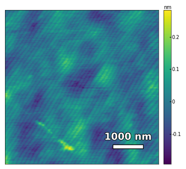
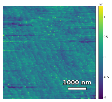
img1 = np.loadtxt('../Data/AFM/untreated_162nm-substrate.txt')[:256]
img1 = np.rot90(img1, k=2)
scalebar_dict = {'image_size': 5000, 'scale_size': 1000, 'units': 'nm'}
visualize_afm_image(img1, colorbar_range=[-4e-10, 4e-10], figsize=(6,4),
                    scalebar_dict=scalebar_dict, filename='untreated_162nm-substrate', printing=printing)
../Figures/2.AFM_XRD/untreated_162nm-substrate.png
../Figures/2.AFM_XRD/untreated_162nm-substrate.svg
../Figures/2.AFM_XRD/untreated_162nm-substrate.tif
img2 = np.loadtxt('../Data/AFM/untreated_162nm-film.txt')[:256]
scalebar_dict = {'image_size': 2008, 'scale_size': 500, 'units': 'nm'}
visualize_afm_image(img2, colorbar_range=[-4e-10, 4e-10], figsize=(6,4),
                    scalebar_dict=scalebar_dict, filename='untreated_162nm-film', printing=printing)
../Figures/2.AFM_XRD/untreated_162nm-film.png
../Figures/2.AFM_XRD/untreated_162nm-film.svg
../Figures/2.AFM_XRD/untreated_162nm-film.tif
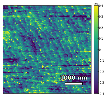
img2 = np.loadtxt('../Data/AFM/untreated_162nm-film.txt')[:256]
scalebar_dict = {'image_size': 2008, 'scale_size': 500, 'units': 'nm'}
visualize_afm_image(img2, colorbar_range=[-4e-10, 4e-10], figsize=(12,8),
                    scalebar_dict=scalebar_dict, filename='untreated_162nm-film-high_res', printing=printing)
../Figures/2.AFM_XRD/untreated_162nm-film-high_res.png
../Figures/2.AFM_XRD/untreated_162nm-film-high_res.svg
../Figures/2.AFM_XRD/untreated_162nm-film-high_res.tif
2.3.2 Calculates the substrate step height, step width, and miscut#
img3 = np.loadtxt('../Data/AFM/untreated_162nm-substrate-tilted.txt')[:256]

scalebar_dict = {'image_size': 5000, 'scale_size': 1000, 'units': 'nm'}
visualize_afm_image(img3, colorbar_range=None, figsize=(6,4), scalebar_dict=scalebar_dict)
# rotate the angle to make step edges horizontal
analyzer = afm_substrate(img3, pixels=256, size=5e-6)
img_rot, size_rot = analyzer.rotate_image(angle=65)

x, z, peak_indices, valley_indices = analyzer.slice_rotate(img_rot, size_rot, j=60, prominence=1e-13, width=2, xz_angle=2, demo=True)
# with the provided height from literature
step_heights, step_widths, miscut = analyzer.calculate_simple(x, z, peak_indices, fixed_height=3.91e-10/2, demo=True)
step_heights, step_widths, miscut = analyzer.calculate_substrate_properties(img_rot, size_rot, xz_angle=2, prominence=1e-13, width=2, style='simple', fixed_height=3.91e-10/2, std_range=1, demo=False)
Step 1: Height = 1.95e-10, Width = 9.41e-08, Miscut = 0.119°
Step 2: Height = 1.95e-10, Width = 9.42e-08, Miscut = 0.119°
Step 3: Height = 1.95e-10, Width = 2.48e-07, Miscut = 0.045°
Step 4: Height = 1.95e-10, Width = 1.30e-07, Miscut = 0.086°
Step 5: Height = 1.95e-10, Width = 1.03e-07, Miscut = 0.109°
Step 6: Height = 1.95e-10, Width = 1.40e-07, Miscut = 0.080°
Step 7: Height = 1.95e-10, Width = 1.09e-07, Miscut = 0.103°
Step 8: Height = 1.95e-10, Width = 1.50e-07, Miscut = 0.075°
Step 9: Height = 1.95e-10, Width = 1.44e-07, Miscut = 0.078°
Step 10: Height = 1.95e-10, Width = 1.47e-07, Miscut = 0.076°
Step 11: Height = 1.95e-10, Width = 1.51e-07, Miscut = 0.074°
Step 12: Height = 1.95e-10, Width = 1.64e-07, Miscut = 0.068°
Step 13: Height = 1.95e-10, Width = 1.29e-07, Miscut = 0.087°
Results:
  Average step height = 1.95e-10, Standard deviation = 0.00e+00
  Average step width = 1.39e-07, Standard deviation = 3.84e-08
  Average miscut = 0.086°, Standard deviation = 0.020°
Step height = 1.95e-10 +- 0.00e+00
Step width = 1.62e-07 +- 8.27e-08
Miscut = 0.090° +- 0.135°
# calculate the height from afm figure
step_heights, step_widths, miscut = analyzer.calculate_simple(x, z, peak_indices, demo=True)
step_heights, step_widths, miscut = analyzer.calculate_substrate_properties(img_rot, size_rot, xz_angle=2, prominence=1e-13, width=2, style='simple', std_range=1, demo=False)
Step 1: Height = 1.17e-10, Width = 9.41e-08, Miscut = 0.071°
Step 2: Height = -7.96e-11, Width = 9.42e-08, Miscut = -0.048°
Step 3: Height = 3.26e-11, Width = 2.48e-07, Miscut = 0.008°
Step 4: Height = -1.59e-10, Width = 1.30e-07, Miscut = -0.070°
Step 5: Height = 3.95e-10, Width = 1.03e-07, Miscut = 0.221°
Step 6: Height = -2.97e-10, Width = 1.40e-07, Miscut = -0.121°
Step 7: Height = 1.14e-10, Width = 1.09e-07, Miscut = 0.060°
Step 8: Height = 1.53e-10, Width = 1.50e-07, Miscut = 0.058°
Step 9: Height = -3.56e-10, Width = 1.44e-07, Miscut = -0.141°
Step 10: Height = -1.48e-12, Width = 1.47e-07, Miscut = -0.001°
Step 11: Height = -4.59e-11, Width = 1.51e-07, Miscut = -0.017°
Step 12: Height = -3.21e-11, Width = 1.64e-07, Miscut = -0.011°
Step 13: Height = 3.85e-11, Width = 1.29e-07, Miscut = 0.017°
Results:
  Average step height = -9.24e-12, Standard deviation = 1.88e-10
  Average step width = 1.39e-07, Standard deviation = 3.84e-08
  Average miscut = 0.002°, Standard deviation = 0.089°
Step height = 2.92e-12 +- 1.98e-10
Step width = 1.62e-07 +- 8.27e-08
Miscut = 0.020° +- 0.260°
x, z, peak_indices, valley_indices = analyzer.slice_rotate(img_rot, size_rot, j=100, prominence=1e-10, width=1, xz_angle=0, demo=True)
step_heights, step_widths, miscut = analyzer.calculate_fit(x, z, peak_indices, valley_indices, fixed_height=3.91e-10/2, demo=True)
step 0: step_width: 2.91e-09, left_peak: (1.62e-07, 1.37e-10), valley: (2.79e-07, -7.53e-11), right_peak: (2.94e-07, 2.61e-10)
step 1: step_width: 6.61e-10, left_peak: (2.94e-07, 2.61e-10), valley: (3.53e-07, -1.69e-10), right_peak: (4.70e-07, 2.93e-10)
step 2: step_width: 7.06e-10, left_peak: (4.70e-07, 2.93e-10), valley: (5.44e-07, -1.95e-10), right_peak: (5.88e-07, -6.45e-11)
step 3: step_width: 3.13e-10, left_peak: (5.88e-07, -6.45e-11), valley: (6.17e-07, -1.77e-10), right_peak: (6.47e-07, 2.45e-11)
step 4: step_width: 2.24e-10, left_peak: (6.47e-07, 2.45e-11), valley: (6.61e-07, -1.39e-10), right_peak: (7.20e-07, 1.04e-10)
step 5: step_width: 4.08e-10, left_peak: (7.20e-07, 1.04e-10), valley: (7.79e-07, -6.47e-11), right_peak: (8.23e-07, 1.15e-10)
step 6: step_width: 3.86e-10, left_peak: (8.23e-07, 1.15e-10), valley: (8.52e-07, -1.05e-10), right_peak: (9.26e-07, 3.10e-10)
step 7: step_width: 2.25e-09, left_peak: (9.26e-07, 3.10e-10), valley: (1.01e-06, -5.36e-10), right_peak: (1.04e-06, -6.95e-11)
step 8: step_width: 2.22e-10, left_peak: (1.04e-06, -6.95e-11), valley: (1.09e-06, -1.74e-10), right_peak: (1.13e-06, -5.75e-11)
step 11: step_width: 6.30e-09, left_peak: (1.32e-06, 1.54e-10), valley: (1.50e-06, -1.42e-10), right_peak: (1.51e-06, 3.58e-10)
step 12: step_width: 8.73e-10, left_peak: (1.51e-06, 3.58e-10), valley: (1.56e-06, -2.73e-11), right_peak: (1.59e-06, 2.98e-10)
step 13: step_width: 9.07e-10, left_peak: (1.59e-06, 2.98e-10), valley: (1.69e-06, -3.23e-10), right_peak: (1.84e-06, 8.45e-11)
step 14: step_width: 4.62e-10, left_peak: (1.84e-06, 8.45e-11), valley: (1.94e-06, -1.68e-10), right_peak: (2.04e-06, 4.15e-11)
step 15: step_width: 1.42e-09, left_peak: (2.04e-06, 4.15e-11), valley: (2.16e-06, -3.13e-10), right_peak: (2.20e-06, 8.66e-11)
step 16: step_width: 5.52e-09, left_peak: (2.20e-06, 8.66e-11), valley: (2.40e-06, -3.71e-10), right_peak: (2.41e-06, 1.87e-11)
step 17: step_width: 4.86e-10, left_peak: (2.41e-06, 1.87e-11), valley: (2.45e-06, -2.14e-10), right_peak: (2.54e-06, 2.92e-10)
step 18: step_width: 1.52e-09, left_peak: (2.54e-06, 2.92e-10), valley: (2.63e-06, -3.69e-11), right_peak: (2.66e-06, 3.61e-10)
step 19: step_width: 1.19e-09, left_peak: (2.66e-06, 3.61e-10), valley: (2.76e-06, -2.50e-10), right_peak: (2.84e-06, 1.63e-10)
step 20: step_width: 1.03e-09, left_peak: (2.84e-06, 1.63e-10), valley: (2.94e-06, -1.20e-10), right_peak: (2.97e-06, 9.47e-11)
step 21: step_width: 3.41e-10, left_peak: (2.97e-06, 9.47e-11), valley: (3.03e-06, -8.17e-11), right_peak: (3.07e-06, 4.20e-11)
step 22: step_width: 4.06e-10, left_peak: (3.07e-06, 4.20e-11), valley: (3.10e-06, -1.61e-10), right_peak: (3.16e-06, 2.45e-10)
Results:
  Average step height = 1.95e-10, Standard deviation = 0.00e+00
  Average step width = 1.36e-09, Standard deviation = 1.62e-09
  Average miscut = 17.713°, Standard deviation = 11.870°
# with the provided height from literature
step_heights, step_widths, miscut = analyzer.calculate_substrate_properties(img_rot, size_rot, xz_angle=0, prominence=1e-10, width=1,
style='fit', fixed_height=3.91e-10/2, std_range=1, demo=False)
Step height = 1.95e-10 +- 2.58e-26
Step width = 8.41e-10 +- 5.97e-10
Miscut = 18.522° +- 10.322°
The “simple” method with provided step height gives a more accurate results for the step width and miscut:
Step height = 1.95e-10 +- 0.00e+00
Step width = 1.62e-07 +- 8.27e-08
Miscut = 0.090° +- 0.135°
3. X-ray Diffraction and Reciprocal Space Mapping#
3.1 \(2\theta\) -\(\omega\) scans#
fig, ax = plt.subplots(1, 1, figsize=(8,3))

files = ['../Data/XRD/substrate-XRD_42_49.xrdml', '../Data/XRD/treated_213nm-XRD_42_29.xrdml',
         '../Data/XRD/treated_81nm-XRD_42_29.xrdml', '../Data/XRD/untreated_162nm-XRD_42_29.xrdml']
labels = ['substrate', 'treated_213nm', 'treated_81nm', 'untreated_162nm']
plot_xrd(ax, files, labels, diff=None, xrange=(41.5, 49.5))
labelfigs(ax, 0, loc='tr', size=15, style='b', inset_fraction=(0.8, 0.1))
Text(48.7, 5391729.771269314, 'a')

3.2 Symmetric Reciprocal Space Mapping (002)#
files = ['../Data/XRD/treated_213nm-RSM_002.xrdml',
         '../Data/XRD/treated_81nm-RSM_002.xrdml',
         '../Data/XRD/untreated_162nm-RSM_002.xrdml']
titles = ['treated_213nm', 'treated_81nm', 'untreated_162nm']

fig, axes = layout_fig(3, 1, figsize=(6,12))
for i, ax in enumerate(axes):
    plot_rsm(ax, files[i], title=titles[i])
    labelfigs(ax, i, loc='tr', size=15)
plt.show()
print(f'\033[1mFig.\033[0m reciprocal space mapping in (002) for sample a: treated_213nm, b: treated_81nm, c: untreated_162nm.')
C:\Users\yig319\Anaconda3\envs\test_rheed\Lib\site-packages\m3util\viz\layout.py:255: UserWarning:

This figure was using a layout engine that is incompatible with subplots_adjust and/or tight_layout; not calling subplots_adjust.

Fig. reciprocal space mapping in (002) for sample a: treated_213nm, b: treated_81nm, c: untreated_162nm.
3.3 Symmetric Reciprocal Space Mapping (103)#
files = ['../Data/XRD/treated_213nm-RSM_103.xrdml',
         '../Data/XRD/treated_81nm-RSM_103.xrdml',
         '../Data/XRD/untreated_162nm-RSM_103.xrdml']
titles = ['treated_213nm', 'treated_81nm', 'untreated_162nm']

fig, axes = layout_fig(3, 1, figsize=(6,15))
for i, ax in enumerate(axes):
    plot_rsm(ax, files[i], title=titles[i])
    labelfigs(ax, i, loc='tr', size=15)
plt.show()
print(f'\033[1mFig.\033[0m reciprocal space mapping in (103) for sample a: treated_213nm, b: treated_81nm, c: untreated_162nm.')

Fig. reciprocal space mapping in (103) for sample a: treated_213nm, b: treated_81nm, c: untreated_162nm.
3.4 Summary Figure of XRD and RSM results#
fig = plt.figure(figsize=(8,8))

ax0 = plt.subplot2grid((4, 2), (0, 0), colspan=2)  # colspan=2 means the plot spans 2 columns
files = ['../Data/XRD/substrate-XRD_42_49.xrdml', '../Data/XRD/treated_213nm-XRD_42_29.xrdml', '../Data/XRD/treated_81nm-XRD_42_29.xrdml', '../Data/XRD/untreated_162nm-XRD_42_29.xrdml']
labels = ['substrate', 'treated_213nm', 'treated_81nm', 'untreated_162nm']
plot_xrd(ax0, files, labels, diff=None, xrange=(44, 48.8), label_size=10, tick_size=8, legend_size=10)
labelfigs(ax0, 0, loc='tr', size=15, style='b', inset_fraction=(0.8, 0.1))

files_002 = ['../Data/XRD/treated_213nm-RSM_002.xrdml', '../Data/XRD/treated_81nm-RSM_002.xrdml', '../Data/XRD/untreated_162nm-RSM_002.xrdml']
for i, file in enumerate(files_002):
    ax = plt.subplot2grid((4, 2), (i+1, 0))
    plot_rsm(ax, file, label_size=10, tick_size=8)
    ax.set_xlim(-0.0032, 0.0032)
    ax.set_ylim(0.505, 0.520)

    labelfigs(ax, i+1, loc='tr', size=15)

files_103 = ['../Data/XRD/treated_213nm-RSM_103.xrdml', '../Data/XRD/treated_81nm-RSM_103.xrdml', '../Data/XRD/untreated_162nm-RSM_103.xrdml']
for i, file in enumerate(files_103):
    ax = plt.subplot2grid((4, 2), (i+1, 1))
    plot_rsm(ax, file, label_size=10, tick_size=8, vmin=3, vmax=1e6)
    ax.set_xlim(0.252, 0.260)
    ax.set_ylim(0.764, 0.773)
    labelfigs(ax, i+4, loc='tr', size=15)

plt.tight_layout()
printing.savefig(fig, 'S2-XRD_RSM')
plt.show()

print(f'\033[1mFig. S2 a\033[0m X-ray Diffraction result for a typical SrTiO3 substrate and samples. \
\033[1mb, c, d\033[0m Reciprocal Space Mapping results in (002) orientaion for sample treated_213nm, treated_81nm and untreated_162nm, respectively. \
\033[1me, f, g\033[0m Reciprocal Space Mapping results in (103) orientaion for sample treated_213nm, treated_81nm and untreated_162nm, respectively.')
../Figures/2.AFM_XRD/S2-XRD_RSM.png
../Figures/2.AFM_XRD/S2-XRD_RSM.svg
../Figures/2.AFM_XRD/S2-XRD_RSM.tif

Fig. S2 a X-ray Diffraction result for a typical SrTiO3 substrate and samples. b, c, d Reciprocal Space Mapping results in (002) orientaion for sample treated_213nm, treated_81nm and untreated_162nm, respectively. e, f, g Reciprocal Space Mapping results in (103) orientaion for sample treated_213nm, treated_81nm and untreated_162nm, respectively.